VisiumHD segmentation

Mar 19, 2025 · 18 min read · Python Spatial Cell Segmentation ·

Spatial transcriptomics reached a whole new level with the latest release from 10x Genomics, Visium HD. This state-of-the-art technology offers exceptional spatial resolution in transcriptomics, enabling researchers to map gene expression with unprecedented detail. From tumor microenvironments to intricate tissue architecture, Visium HD is transforming cellular biology experiments— pixel by pixel.

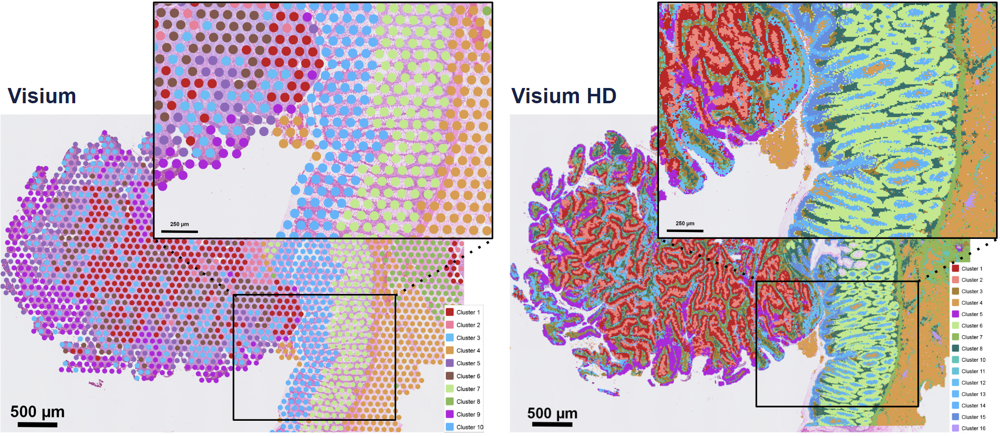
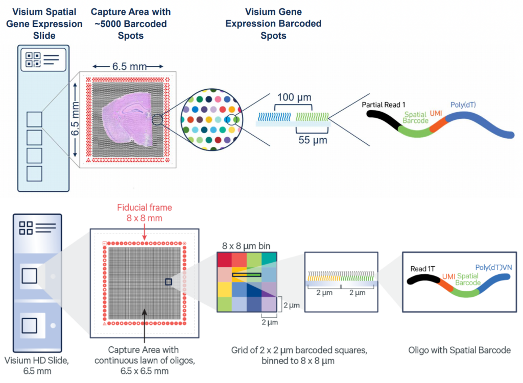
Visium v2 data (left) and Visium HD data (right) in FFPE human colorectal cancer. Credit 10Xgenomics.com

The key advantage of Visium HD over Visium is moving from discrete spots to a continuous lawn of oligonucleotides arrayed into millions of 2 x 2 µm barcoded squares that captures whole transcriptome expression.

Visium (top) and Visium HD (bottom) slide capture area structure. Credit 10Xgenomics.com

Eventhough Visium HD provides extreme resolution, we still miss a key part to truly understand the biology of the system: single-cell individuality. Luckily for us, we can use segmentation techniques to reconstructs cells from the high resolution Visium HD data.

In today's post we will start using a 'simple' approach of nuclei segmentation following this 10X Genomics tutorial

Input data

We will use the 10x Mouse Small Intestine (FFPE) dataset, especifically the following data:

2x2 µm filtered barcode matrix (filtered_feature_bc_matrix.h5)
Parquet tissue position matrix (tissue_positions.parquet)
High-resolution mouse intestine image (Visium_HD_Mouse_Small_Intestine_tissue_image.btf)

Download the data from 10X website and extract the files.

1curl -O https://cf.10xgenomics.com/samples/spatial-exp/3.0.0/Visium_HD_Mouse_Small_Intestine/Visium_HD_Mouse_Small_Intestine_binned_outputs.tar.gz
2curl -O https://cf.10xgenomics.com/samples/spatial-exp/3.0.0/Visium_HD_Mouse_Small_Intestine/Visium_HD_Mouse_Small_Intestine_tissue_image.btf

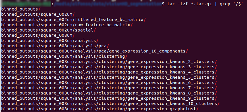
show tar contents (only folders)

1tar -tf Visium_HD_Mouse_Small_Intestine_binned_outputs.tar.gz | grep '/$'

Let's start by loading the required packages.

 1import pandas as pd
 2import numpy as np
 3import matplotlib.pyplot as plt
 4import anndata
 5import geopandas as gpd
 6import scanpy as sc
 7from tifffile import imread, imwrite
 8from csbdeep.utils import normalize
 9from stardist.models import StarDist2D
10from shapely.geometry import Polygon, Point
11from scipy import sparse
12from matplotlib.colors import ListedColormap
13
14# Configuration for inline plotting
15%matplotlib inline
16%config InlineBackend.figure_format = 'retina'

2025-01-22 17:46:53.617273: I tensorflow/core/platform/cpu_feature_guard.cc:182] This TensorFlow binary is optimized to use available CPU instructions in performance-critical operations.
To enable the following instructions: AVX2 FMA, in other operations, rebuild TensorFlow with the appropriate compiler flags.

TensorFlow complains a little bit but it works.

The following code defines some utility functions, you can skip it and come back later if are curious or have questions.

  1# General image plotting functions
  2def plot_mask_and_save_image(title, gdf, img, cmap, output_name=None, bbox=None):
  3    if bbox is not None:
  4        # Crop the image to the bounding box
  5        cropped_img = img[bbox[1]:bbox[3], bbox[0]:bbox[2]]
  6    else:
  7        cropped_img = img
  8
  9    # Plot options
 10    fig, axes = plt.subplots(1, 2, figsize=(12, 6))
 11
 12    # Plot the cropped image
 13    axes[0].imshow(cropped_img, cmap='gray', origin='lower')
 14    axes[0].set_title(title)
 15    axes[0].axis('off')
 16
 17    # Create filtering polygon
 18    if bbox is not None:
 19        bbox_polygon = Polygon([(bbox[0], bbox[1]), (bbox[2], bbox[1]), (bbox[2], bbox[3]), (bbox[0], bbox[3])])
 20        # Filter for polygons in the box
 21        intersects_bbox = gdf['geometry'].intersects(bbox_polygon)
 22        filtered_gdf = gdf[intersects_bbox]
 23    else:
 24        filtered_gdf=gdf
 25
 26    # Plot the filtered polygons on the second axis
 27    filtered_gdf.plot(cmap=cmap, ax=axes[1])
 28    axes[1].axis('off')
 29    axes[1].legend(loc='upper left', bbox_to_anchor=(1.05, 1))
 30
 31
 32    # Save the plot if output_name is provided
 33    if output_name is not None:
 34        plt.savefig(output_name, bbox_inches='tight')  # Use bbox_inches='tight' to include the legend
 35    else:
 36        plt.show()
 37
 38def plot_gene_and_save_image(title, gdf, gene, img, adata, bbox=None, output_name=None):
 39
 40    if bbox is not None:
 41        # Crop the image to the bounding box
 42        cropped_img = img[bbox[1]:bbox[3], bbox[0]:bbox[2]]
 43    else:
 44        cropped_img = img
 45
 46    # Plot options
 47    fig, axes = plt.subplots(1, 2, figsize=(12, 6))
 48
 49    # Plot the cropped image
 50    axes[0].imshow(cropped_img, cmap='gray', origin='lower')
 51    axes[0].set_title(title)
 52    axes[0].axis('off')
 53
 54    # Create filtering polygon
 55    if bbox is not None:
 56        bbox_polygon = Polygon([(bbox[0], bbox[1]), (bbox[2], bbox[1]), (bbox[2], bbox[3]), (bbox[0], bbox[3])])
 57
 58
 59    # Find a gene of interest and merge with the geodataframe
 60    gene_expression = adata[:, gene].to_df()
 61    gene_expression['id'] = gene_expression.index
 62    merged_gdf = gdf.merge(gene_expression, left_on='id', right_on='id')
 63
 64    if bbox is not None:
 65        # Filter for polygons in the box
 66        intersects_bbox = merged_gdf['geometry'].intersects(bbox_polygon)
 67        filtered_gdf = merged_gdf[intersects_bbox]
 68    else:
 69        filtered_gdf = merged_gdf
 70
 71    # Plot the filtered polygons on the second axis
 72    filtered_gdf.plot(column=gene, cmap='inferno', legend=True, ax=axes[1])
 73    axes[1].set_title(gene)
 74    axes[1].axis('off')
 75    axes[1].legend(loc='upper left', bbox_to_anchor=(1.05, 1))
 76
 77    # Save the plot if output_name is provided
 78    if output_name is not None:
 79        plt.savefig(output_name, bbox_inches='tight')  # Use bbox_inches='tight' to include the legend
 80    else:
 81        plt.show()
 82
 83def plot_clusters_and_save_image(title, gdf, img, adata, bbox=None, 
 84                                 color_by_obs=None, output_name=None, color_list=None):
 85    color_list=["#7f0000","#808000","#483d8b","#008000","#bc8f8f","#008b8b","#4682b4","#000080","#d2691e","#9acd32","#8fbc8f","#800080","#b03060","#ff4500","#ffa500","#ffff00","#00ff00","#8a2be2","#00ff7f","#dc143c","#00ffff","#0000ff","#ff00ff","#1e90ff","#f0e68c","#90ee90","#add8e6","#ff1493","#7b68ee","#ee82ee"]
 86    if bbox is not None:
 87        cropped_img = img[bbox[1]:bbox[3], bbox[0]:bbox[2]]
 88    else:
 89        cropped_img = img
 90
 91    fig, axes = plt.subplots(1, 2, figsize=(12, 6))
 92
 93    axes[0].imshow(cropped_img, cmap='gray', origin='lower')
 94    axes[0].set_title(title)
 95    axes[0].axis('off')
 96
 97    if bbox is not None:
 98        bbox_polygon = Polygon([(bbox[0], bbox[1]), (bbox[2], bbox[1]), (bbox[2], bbox[3]), (bbox[0], bbox[3])])
 99
100    unique_values = adata.obs[color_by_obs].astype('category').cat.categories
101    num_categories = len(unique_values)
102
103    if color_list is not None and len(color_list) >= num_categories:
104        custom_cmap = ListedColormap(color_list[:num_categories], name='custom_cmap')
105    else:
106        # Use default tab20 colors if color_list is insufficient
107        tab20_colors = plt.cm.tab20.colors[:num_categories]
108        custom_cmap = ListedColormap(tab20_colors, name='custom_tab20_cmap')
109
110    merged_gdf = gdf.merge(adata.obs[color_by_obs].astype('category'), left_on='id', right_index=True)
111
112    if bbox is not None:
113        intersects_bbox = merged_gdf['geometry'].intersects(bbox_polygon)
114        filtered_gdf = merged_gdf[intersects_bbox]
115    else:
116        filtered_gdf = merged_gdf
117
118    # Plot the filtered polygons on the second axis
119    plot = filtered_gdf.plot(column=color_by_obs, cmap=custom_cmap, ax=axes[1], legend=True)
120    axes[1].set_title(color_by_obs)
121    legend = axes[1].get_legend()
122    legend.set_bbox_to_anchor((1.05, 1))
123    axes[1].axis('off')
124
125    # Move legend outside the plot
126    plot.get_legend().set_bbox_to_anchor((1.25, 1))
127
128    if output_name is not None:
129        plt.savefig(output_name, bbox_inches='tight')
130    else:
131        plt.show()
132
133# Plotting function for nuclei area distribution
134def plot_nuclei_area(gdf,area_cut_off):
135    fig, axs = plt.subplots(1, 2, figsize=(15, 4))
136    # Plot the histograms
137    axs[0].hist(gdf['area'], bins=50, edgecolor='black')
138    axs[0].set_title('Nuclei Area')
139
140    axs[1].hist(gdf[gdf['area'] < area_cut_off]['area'], bins=50, edgecolor='black')
141    axs[1].set_title('Nuclei Area Filtered:'+str(area_cut_off))
142
143    plt.tight_layout()
144    plt.show()
145
146# Total UMI distribution plotting function
147def total_umi(adata_, cut_off):
148    fig, axs = plt.subplots(1, 2, figsize=(12, 4))
149
150    # Box plot
151    axs[0].boxplot(adata_.obs["total_counts"], vert=False, widths=0.7, patch_artist=True, boxprops=dict(facecolor='skyblue'))
152    axs[0].set_title('Total Counts')
153
154    # Box plot after filtering
155    axs[1].boxplot(adata_.obs["total_counts"][adata_.obs["total_counts"] > cut_off], vert=False, widths=0.7, patch_artist=True, boxprops=dict(facecolor='skyblue'))
156    axs[1].set_title('Total Counts > ' + str(cut_off))
157
158    # Remove y-axis ticks and labels
159    for ax in axs:
160        ax.get_yaxis().set_visible(False)
161
162    plt.tight_layout()
163    plt.show()
164    
165# coexpression summary
166def calculate_summary(adata, gene_names):
167    """
168    Calculate the summary of the number of rows with both genes' expression == 0,
169    each of the genes' expression == 0, and none of the genes' expression == 0.
170    
171    Parameters:
172    - adata: AnnData object
173    - gene_names: list of two gene names (strings)
174    
175    Returns:
176    - summary: dictionary containing the counts
177    """
178    gene1, gene2 = gene_names
179
180    # Get the indices of the genes
181    col1 = adata.var_names.get_loc(gene1)
182    col2 = adata.var_names.get_loc(gene2)
183    
184    # Extract the expression data for the two genes
185    expr_data = adata.X[:, [col1, col2]].toarray()
186    
187    both_zero = np.sum((expr_data[:, 0] == 0) & (expr_data[:, 1] == 0))
188    gene1_zero = np.sum((expr_data[:, 0] == 0) & (expr_data[:, 1] != 0))
189    gene2_zero = np.sum((expr_data[:, 0] != 0) & (expr_data[:, 1] == 0))
190    none_zero = np.sum((expr_data[:, 0] != 0) & (expr_data[:, 1] != 0))
191    
192    summary = {
193        'both_zero': both_zero,
194        'gene1_zero': gene1_zero,
195        'gene2_zero': gene2_zero,
196        'none_zero': none_zero
197    }
198    
199    return summary

Nuclei Segmentation

Image preparation

We start loading the H&E image

1filename = 'Visium_HD_Mouse_Small_Intestine_tissue_image.btf'
2img = imread(filename)

and then check it

1plt.figure(figsize=(10, 10))
2plt.imshow(img)
3# plt.axis('off')  # Uncomment to hide the axis
4plt.show()

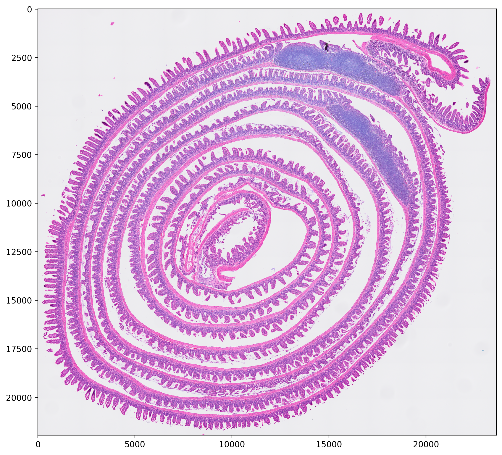
and print some information about the image

1print("Image shape:", img.shape)
2print("Image dtype:", img.dtype)

Image shape: (21943, 23618, 3)
Image dtype: uint8

Next we load the pretrained model to find the nuclei in the H&E image.

1model = StarDist2D.from_pretrained('2D_versatile_he')

Found model '2D_versatile_he' for 'StarDist2D'.
Downloading data from https://github.com/stardist/stardist-models/releases/download/v0.1/python_2D_versatile_he.zip
5294730/5294730 [==============================] - 0s 0us/step    

2025-01-22 17:52:50.985061: I tensorflow/core/common_runtime/gpu/gpu_device.cc:1639] Created device /job:localhost/replica:0/task:0/device:GPU:0 with 6308 MB memory:  -> device: 0, name: NVIDIA GeForce RTX 2070 SUPER, pci bus id: 0000:01:00.0, compute capability: 7.5


Loading network weights from 'weights_best.h5'.
Loading thresholds from 'thresholds.json'.
Using default values: prob_thresh=0.692478, nms_thresh=0.3.

Before prediction, the H&E image must be normalized. We use the percentile normalization, which scales pixel values by the specified min and max percentiles. These values may need to be adjusted as needed for other images based on the nuclei predictions.

1min_percentile = 5
2max_percentile = 95
3img = normalize(img, min_percentile, max_percentile)

Nuclei prediction

With the pretrained model and the normalized image we can start the nuclei prediction. This step may take a long time and it is the reason we need to use a GPU.

1labels, polys = model.predict_instances_big(img, axes='YXC', block_size=4096,
2                                            prob_thresh=0.01, nms_thresh=0.001,
3                                            min_overlap=128, context=128,
4                                            normalizer=None, n_tiles=(4,4,1))

effective: block_size=(4096, 4096, 3), min_overlap=(128, 128, 0), context=(128, 128, 0)


2025-01-22 17:53:25.169612: I tensorflow/compiler/xla/stream_executor/cuda/cuda_dnn.cc:432] Loaded cuDNN version 8600
100%|████████████████████████████████████████████████████████████████████| 42/42 [05:58<00:00,  8.52s/it]

Let's understand the ouput:

block_size: The size of the blocks (or tiles) into which the large image is divided for processing. Each block has dimensions of 4096 pixels by 4096 pixels with 3 channels (RGB).
min_overlap: Minimum overlap between adjacent blocks to ensure that objects that lie on the boundaries of blocks are properly segmented. Set to 128 pixels in both the x and y directions, and no overlap in the channel dimension.
context: Context size around each block considered during processing. It helps in providing additional information from the surrounding areas of a block. Set to 128 pixels around each block in both the x and y directions.

StarDist package provides two functions to predict nuclei, predict_instances and predict_instances_big, the second one divides the original image in blocks to perform the prediction and then combines the results. The following parameters may need to be adjusted based on the results:

prob_thresh: Probability threshold to remove low-confidence object predictions.
nms_thresh: Overlap threshold to perform non-maximum suppression.

The next code will generate a Geodataframe to store the nuclei predictions, it will be used to filter the VisiumHD barcodes.

 1# Creating a list to store Polygon geometries
 2geometries = []
 3
 4# Iterating through each nuclei in the 'polys' DataFrame
 5for nuclei in range(len(polys['coord'])):
 6
 7    # Extracting coordinates for the current nuclei and converting them to (y, x) format
 8    coords = [(y, x) for x, y in zip(polys['coord'][nuclei][0], polys['coord'][nuclei][1])]
 9
10    # Creating a Polygon geometry from the coordinates
11    geometries.append(Polygon(coords))
12
13# Creating a GeoDataFrame using the Polygon geometries
14gdf = gpd.GeoDataFrame(geometry=geometries)
15gdf['id'] = [f"ID_{i+1}" for i, _ in enumerate(gdf.index)]

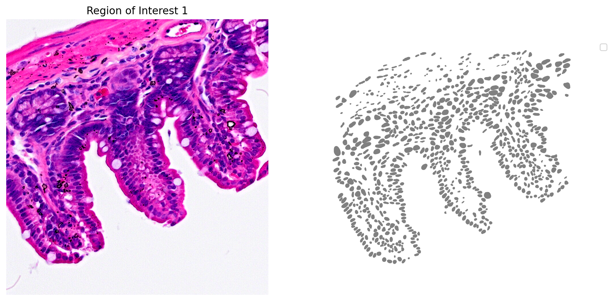
Let's check the predictions in a region of interest (ROI)

1# Define a single color cmap
2cmap=ListedColormap(['grey'])
3
4# Create Plot
5plot_mask_and_save_image(title="Region of Interest 1", gdf=gdf,
6                         bbox=(12844,7700,13760,8664), cmap=cmap,
7                         img=img)

Clipping input data to the valid range for imshow with RGB data ([0..1] for floats or [0..255] for integers).
No artists with labels found to put in legend.  Note that artists whose label start with an underscore are ignored when legend() is called with no argument.

Filter Visium HD Barcodes

We start by loading the 2x2 µm filtered barcode matrix

1dir_base = '/tf/visium/binned_outputs/square_002um/'
2raw_h5_file = dir_base+'filtered_feature_bc_matrix.h5'
3adata = sc.read_10x_h5(raw_h5_file)

anndata.py (1840): Variable names are not unique. To make them unique, call `.var_names_make_unique`.
anndata.py (1840): Variable names are not unique. To make them unique, call `.var_names_make_unique`.

annData complains about duplicated variable names, let's take a look.

1# check var_names
2adata.var_names

Index(['Xkr4', 'Rp1', 'Sox17', 'Lypla1', 'Tcea1', 'Rgs20', 'Atp6v1h', 'Oprk1',
       'Npbwr1', 'Rb1cc1',
       ...
       'mt-Atp8', 'mt-Atp6', 'mt-Co3', 'mt-Nd3', 'mt-Nd4l', 'mt-Nd4', 'mt-Nd5',
       'mt-Nd6', 'mt-Cytb', 'Vamp7'],
      dtype='object', length=19059)

their number,

1len( adata.var_names.tolist() )

and the unique gene names length

1len( set( adata.var_names.tolist() ) )

Let's make the variable (gene) names unique

1# Make variable names unique
2adata.var_names_make_unique()

and check dimensions to confirm we did not loose any gene

1adata.shape

(5479660, 19059)

Next we load the spatial coordinates of the barcodes

1tissue_position_file = dir_base+'spatial/'+'tissue_positions.parquet'
2df_tissue_positions=pd.read_parquet(tissue_position_file)

and add it to the annData object

1#Set the index of the dataframe to the barcodes
2df_tissue_positions = df_tissue_positions.set_index('barcode')
3# Create an index in the dataframe to check joins
4df_tissue_positions['index']=df_tissue_positions.index
5# Adding the tissue positions to the meta data
6adata.obs =  pd.merge(adata.obs, df_tissue_positions, left_index=True, right_index=True)

Next steps is creating a GeoDataFrame to store the spatial information.

1geometry = [Point(xy) for xy in zip(df_tissue_positions['pxl_col_in_fullres'], df_tissue_positions['pxl_row_in_fullres'])]
2gdf_coordinates = gpd.GeoDataFrame(df_tissue_positions, geometry=geometry)

We use it to identify the barcodes belonging to cell nuclei. We also remove overlapping nuclei to keep barcodes that are uniquely assigned and generate a new annData object.

 1# Perform a spatial join to check which coordinates are in a cell nucleus
 2result_spatial_join = gpd.sjoin(gdf_coordinates, gdf, how='left', predicate='within')
 3# Identify nuclei associated barcodes and find barcodes that are in more than one nucleus
 4result_spatial_join['is_within_polygon'] = ~result_spatial_join['index_right'].isna()
 5barcodes_in_overlaping_polygons = pd.unique(result_spatial_join[result_spatial_join.duplicated(subset=['index'])]['index'])
 6result_spatial_join['is_not_in_an_polygon_overlap'] = ~result_spatial_join['index'].isin(barcodes_in_overlaping_polygons)
 7# Remove barcodes in overlapping nuclei
 8barcodes_in_one_polygon = result_spatial_join[result_spatial_join['is_within_polygon'] & result_spatial_join['is_not_in_an_polygon_overlap']]
 9# The AnnData object is filtered to only contain the barcodes that are in non-overlapping polygon regions
10filtered_obs_mask = adata.obs_names.isin(barcodes_in_one_polygon['index'])
11filtered_adata = adata[filtered_obs_mask,:]
12# Add the results of the point spatial join to the Anndata object
13filtered_adata.obs =  pd.merge(filtered_adata.obs, barcodes_in_one_polygon[['index','geometry','id','is_within_polygon','is_not_in_an_polygon_overlap']], left_index=True, right_index=True)

The final step is calculating the gene count summation of the nuclei.

 1# Group the data by unique nucleous IDs
 2groupby_object = filtered_adata.obs.groupby(['id'], observed=True)
 3# Extract the gene expression counts from the AnnData object
 4counts = filtered_adata.X
 5# Obtain the number of unique nuclei and the number of genes in the expression data
 6N_groups = groupby_object.ngroups
 7N_genes = counts.shape[1]
 8# Initialize a sparse matrix to store the summed gene counts for each nucleus
 9summed_counts = sparse.lil_matrix((N_groups, N_genes))
10# Lists to store the IDs of polygons and the current row index
11polygon_id = []
12row = 0
13# Iterate over each unique polygon to calculate the sum of gene counts.
14for polygons, idx_ in groupby_object.indices.items():
15    summed_counts[row] = counts[idx_].sum(0)
16    row += 1
17    polygon_id.append(polygons)
18# Create and AnnData object from the summed count matrix
19summed_counts = summed_counts.tocsr()
20grouped_filtered_adata = anndata.AnnData(X=summed_counts,obs=pd.DataFrame(polygon_id,columns=['id'],index=polygon_id),var=filtered_adata.var)

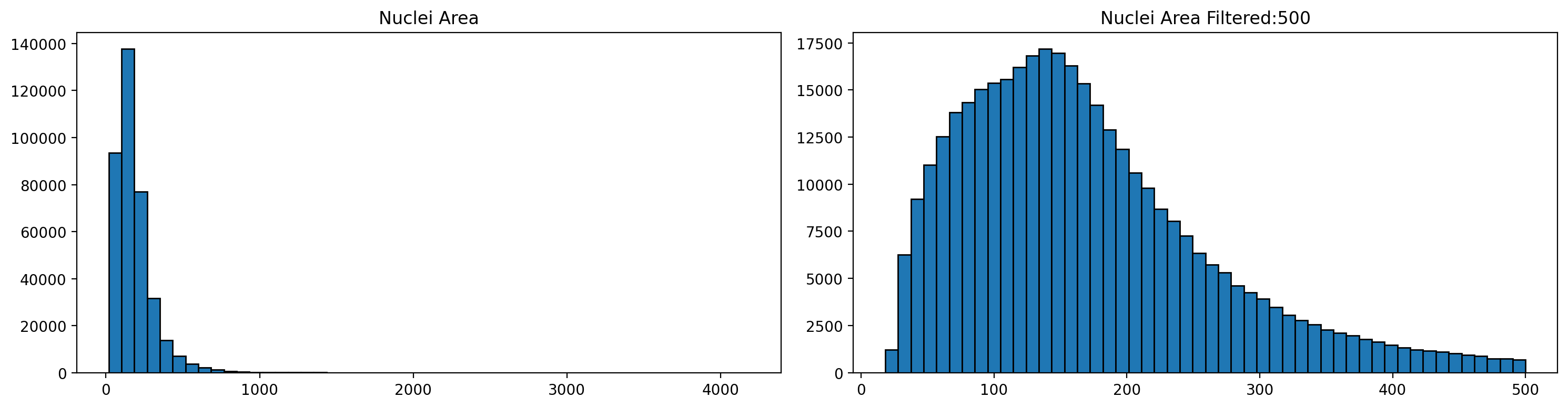
Nuclei filtering

We filter the largest nuclei as they likely correspond to aggregates or artifacts. We also remove nuclei with low total umi counts, as we would do in a single cell RNAseq experiment.

Let's check size distribution (left) and the results filtering over a 500 cutoff (rigth)

1# Store the area of each nucleus in the GeoDataframe
2gdf['area'] = gdf['geometry'].area
3
4
5# Plot the nuclei area distribution before and after filtering
6plot_nuclei_area(gdf=gdf,area_cut_off=500)

Now let's focus on total UMI count distribution (left) and filtering with a 100 threshold.

1# Calculate quality control metrics for the original AnnData object
2sc.pp.calculate_qc_metrics(grouped_filtered_adata, inplace=True)
3
4# Plot total UMI distribution
5total_umi(grouped_filtered_adata, 100)

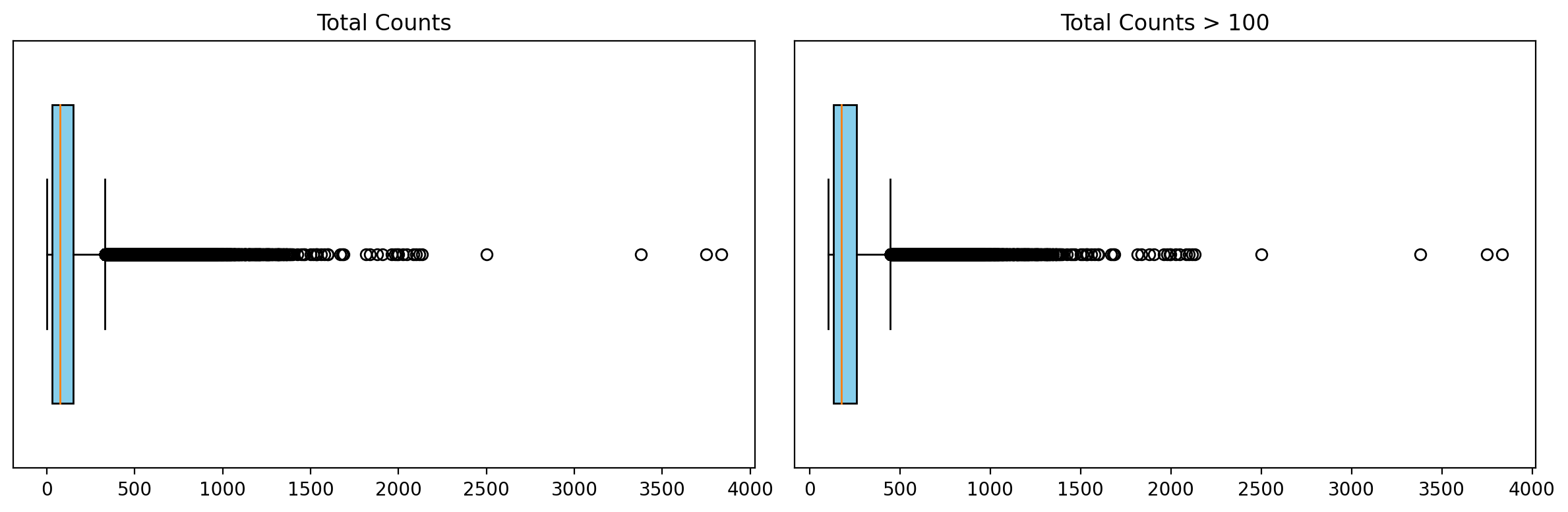
The thresholds to apply will vary depending on the dataset and experiment. Selecting appropriate thresholds takes experience and evaluation of downstream analyses such us clustering or marker gene expression.

Let's perform the actual filtering and calculate some quality control metrics.

 1# Create a mask based on the 'id' column for values present in 'gdf' with 'area' less than 500
 2mask_area = grouped_filtered_adata.obs['id'].isin(gdf[gdf['area'] < 500].id)
 3
 4# Create a mask based on the 'total_counts' column for values greater than 100
 5mask_count = grouped_filtered_adata.obs['total_counts'] > 100
 6
 7# Apply both masks to the original AnnData to create a new filtered AnnData object
 8count_area_filtered_adata = grouped_filtered_adata[mask_area & mask_count, :]
 9
10# Calculate quality control metrics for the filtered AnnData object
11sc.pp.calculate_qc_metrics(count_area_filtered_adata, inplace=True)

_qc.py (135): Trying to modify attribute `.obs` of view, initializing view as actual.

Clustering

The following code performs a typical single cell RNAseq analysis pipeline, from normalization to clustering, using scanpy.

 1# Normalize total counts for each cell in the AnnData object
 2sc.pp.normalize_total(count_area_filtered_adata, inplace=True)
 3
 4# Logarithmize the values in the AnnData object after normalization
 5sc.pp.log1p(count_area_filtered_adata)
 6
 7# Identify highly variable genes in the dataset using the Seurat method
 8sc.pp.highly_variable_genes(count_area_filtered_adata, flavor="seurat", n_top_genes=2000)
 9
10# Perform Principal Component Analysis (PCA) on the AnnData object
11sc.pp.pca(count_area_filtered_adata)
12
13# Build a neighborhood graph based on PCA components
14sc.pp.neighbors(count_area_filtered_adata)
15
16# Perform Leiden clustering on the neighborhood graph and store the results in 'clusters' column
17sc.tl.leiden(count_area_filtered_adata, resolution=0.35, key_added="clusters")

now we can check the results. We will do it in a ROI (Region Of Interest) for the shake of simplicity.

1plot_clusters_and_save_image(title="Region of interest 1", 
2                             gdf=gdf, img=img, adata=count_area_filtered_adata, 
3                             bbox=(12844,7700,13760,8664), color_by_obs='clusters')

Clipping input data to the valid range for imshow with RGB data ([0..1] for floats or [0..255] for integers).

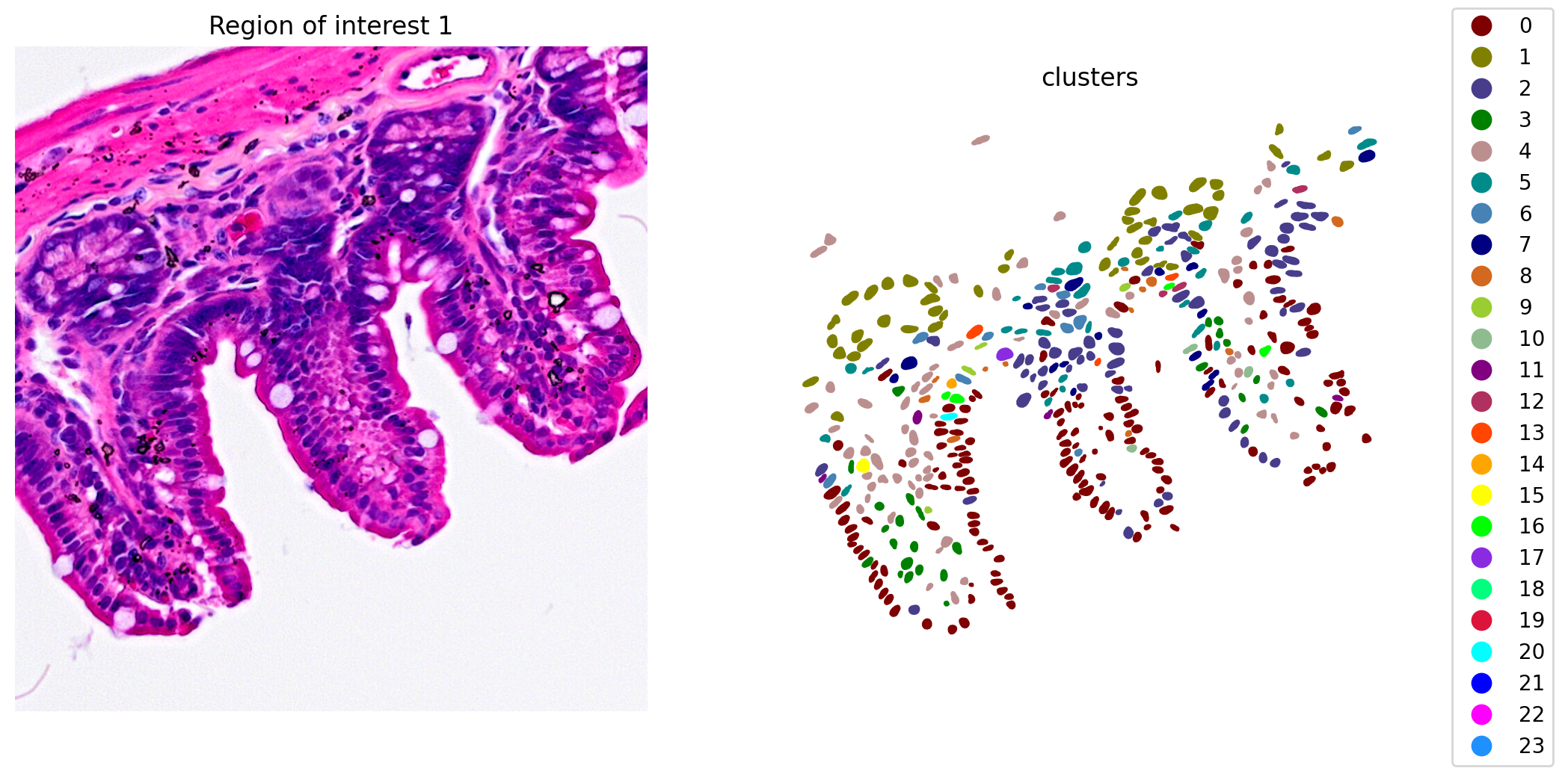
We got 24 clusters that seem to group pretty well different cell types.

Marker Genes

Let's see how behave some specific cell type marker genes:

Paneth cell: Lyz1
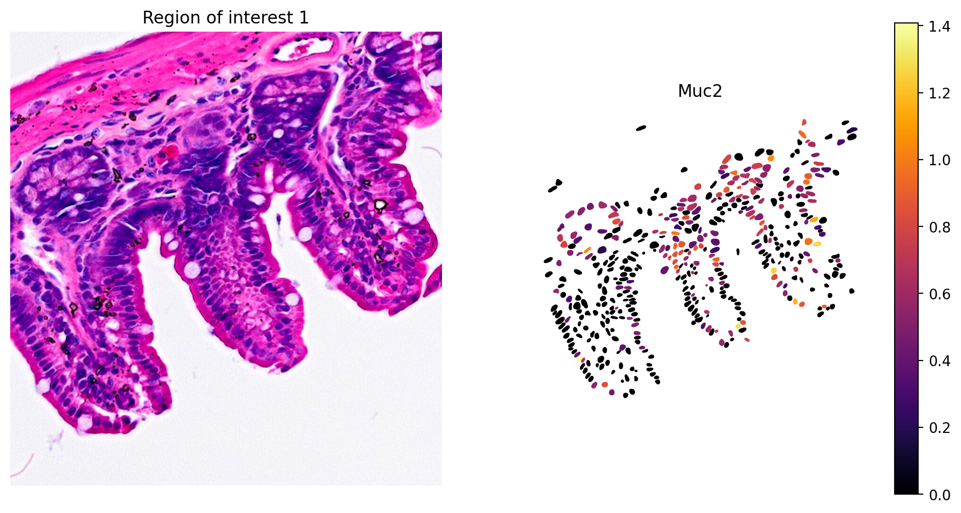
Goblet cell: Muc2
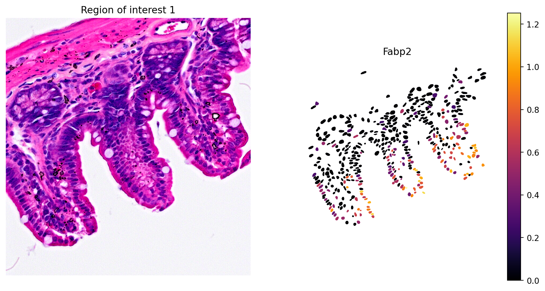
Enterocyte cell: Fabp2
Plasma cell: Jchain

Paneth cells

1plot_gene_and_save_image(title="Region of interest 1", 
2                         gdf=gdf, gene='Lyz1', img=img, 
3                         adata=count_area_filtered_adata, 
4                         bbox=(12844,7700,13760,8664))

Clipping input data to the valid range for imshow with RGB data ([0..1] for floats or [0..255] for integers).
No artists with labels found to put in legend.  Note that artists whose label start with an underscore are ignored when legend() is called with no argument.

Goblet cells

1plot_gene_and_save_image(title="Region of interest 1", gdf=gdf, gene='Muc2', 
2                         img=img, adata=count_area_filtered_adata, bbox=(12844,7700,13760,8664))

Clipping input data to the valid range for imshow with RGB data ([0..1] for floats or [0..255] for integers).
No artists with labels found to put in legend.  Note that artists whose label start with an underscore are ignored when legend() is called with no argument.

Enterocyte cells

1plot_gene_and_save_image(title="Region of interest 1", gdf=gdf, gene='Fabp2', 
2                         img=img, adata=count_area_filtered_adata, bbox=(12844,7700,13760,8664))

Clipping input data to the valid range for imshow with RGB data ([0..1] for floats or [0..255] for integers).
No artists with labels found to put in legend.  Note that artists whose label start with an underscore are ignored when legend() is called with no argument.

Plasma cells

1plot_gene_and_save_image(title="Region of interest 1", gdf=gdf, gene='Jchain', 
2                         img=img, adata=count_area_filtered_adata, bbox=(12844,7700,13760,8664))

Clipping input data to the valid range for imshow with RGB data ([0..1] for floats or [0..255] for integers).
No artists with labels found to put in legend.  Note that artists whose label start with an underscore are ignored when legend() is called with no argument.

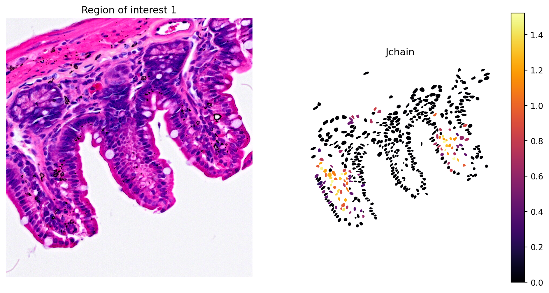
The marker analysis in the ROI seems quite good.

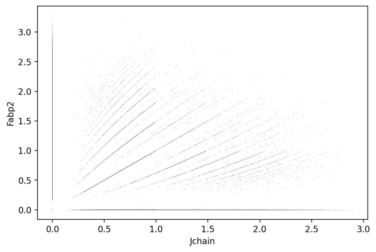
Segmentation analysis

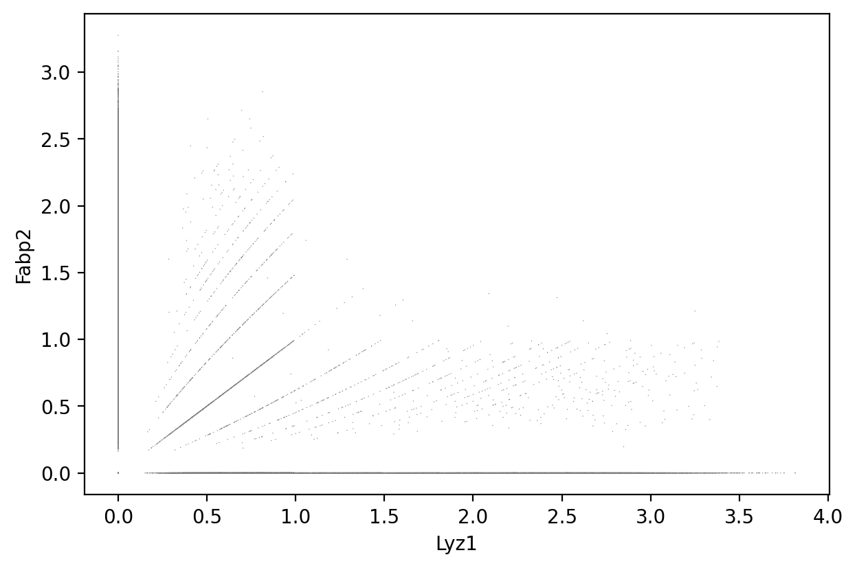
One of the main issues when doing segmentation analyses is mixing cell types in the process. Although here we are on the safe side since we are segmenting nuclei, we will test for cell type marker coexpression slide-wide using scatter plots.

Lyz1 and Fabp2

1sc.pl.scatter(count_area_filtered_adata, x = 'Lyz1', y = 'Fabp2' )

 1gene_markers = ['Lyz1', 'Fabp2']
 2summary = calculate_summary(count_area_filtered_adata, gene_markers )
 3total = sum(summary.values())
 4percentages = {key: (value / total) * 100 for key, value in summary.items()}
 5print( "Double negative: {:.2f}%\n{} positive: {:.2f}%\n{} positive: {:.2f}%\nDouble positive: {:.2f}%".format(
 6    percentages['both_zero'],
 7    gene_markers[1], percentages['gene1_zero'],
 8    gene_markers[0], percentages['gene2_zero'],
 9    percentages['none_zero']
10) )

Double negative: 50.98%
Fabp2 positive: 32.07%
Lyz1 positive: 15.36%
Double positive: 1.59%

Lyz1 and Jchain

1sc.pl.scatter(count_area_filtered_adata, x = 'Lyz1', y = 'Jchain' )

 1gene_markers = ['Lyz1', 'Jchain']
 2summary = calculate_summary(count_area_filtered_adata, gene_markers )
 3total = sum(summary.values())
 4percentages = {key: (value / total) * 100 for key, value in summary.items()}
 5print( "Double negative: {:.2f}%\n{} positive: {:.2f}%\n{} positive: {:.2f}%\nDouble positive: {:.2f}%".format(
 6    percentages['both_zero'],
 7    gene_markers[1], percentages['gene1_zero'],
 8    gene_markers[0], percentages['gene2_zero'],
 9    percentages['none_zero']
10) )

Double negative: 68.62%
Jchain positive: 14.43%
Lyz1 positive: 15.10%
Double positive: 1.85%

Jchain and Fabp2

1sc.pl.scatter(count_area_filtered_adata, x = 'Jchain', y = 'Fabp2' )

 1gene_markers = ['Jchain', 'Fabp2']
 2summary = calculate_summary(count_area_filtered_adata, gene_markers )
 3total = sum(summary.values())
 4percentages = {key: (value / total) * 100 for key, value in summary.items()}
 5print( "Double negative: {:.2f}%\n{} positive: {:.2f}%\n{} positive: {:.2f}%\nDouble positive: {:.2f}%".format(
 6    percentages['both_zero'],
 7    gene_markers[1], percentages['gene1_zero'],
 8    gene_markers[0], percentages['gene2_zero'],
 9    percentages['none_zero']
10) )

Double negative: 55.20%
Fabp2 positive: 28.52%
Jchain positive: 11.15%
Double positive: 5.13%

Cluster annotation

Once we are happy with our segmentation results we can go ahead and annotate (assign a cell type) our clusters. There are many ways of doing this, we will do it assessing cell type marker expression with a dot plot.

Dot plots shows gene expression level (color intensity) and the percentage of expressing cells (dot size) for selected genes across cell groups, clusters in this case. Larger, darker dots indicate stronger and more widespread expression, helping to identify which clusters correspond to specific cell types.

1markers = ['Lyz1', 'Muc2', 'Jchain', 'Fabp2']
2sc.pl.dotplot(count_area_filtered_adata, markers, groupby='clusters', dendrogram=True)

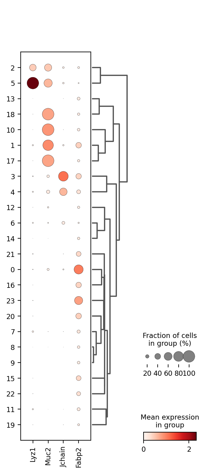
It seems cluster 5 corresponds to Paneth cells; clusters 1, 10, 17, and 18 to Goblet cells; clusters 3 and 4 to Plasma cells; and clusters 0, 16, 20, and 23 to Enterocytes. However, many clusters remain unidentified. Lets try to identify some immune system cell types, T-cells and macrophages. We will also add more information to the dotplot.

1# cd64: FCGR1. Intestinal macrophages markers https://pmc.ncbi.nlm.nih.gov/articles/PMC4451680/ 
2markers = { 'Paneth': 'Lyz1', 'Goblet': 'Muc2', 'Plasma Cell': 'Jchain', 'Enterocyte': 'Fabp2', 'T-cells': [ 'Cd3' + l for l in 'de' ], 'Macrophages': [ 'Fcgr1', 'Adgre1', 'Cd68' ] }
3p = sc.pl.dotplot(count_area_filtered_adata, markers, groupby='clusters', dendrogram=True, return_fig=True)
4p.add_totals().style(dot_edge_color='black', dot_edge_lw=0.5).show()

WARNING: Groups are not reordered because the `groupby` categories and the `var_group_labels` are different.
categories: 0, 1, 2, etc.
var_group_labels: Paneth, Goblet, Plasma Cell, etc.

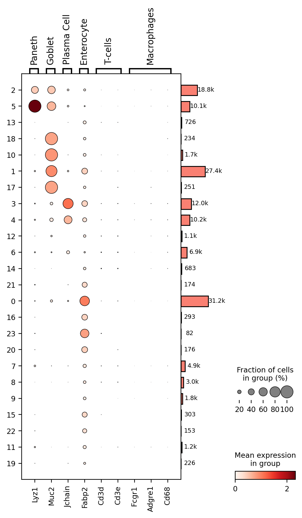
Apparently there are no T-cells or Macrophagues in this dataset, although most of these markers came from the FACS cell selection and it is well known that these type of markers are often not very useful in transcriptomics approaches. Here is where multimodal approaches, combining protein and RNA detection become very useful. Another alternative is searching the literature to find useful markers for these cell types at the transcriptomic level. Which markers would you use? Let's us know in the comments section below.

The lateral bars indicate the number of cells in each and are useful to understand their importance since it is not the same a cluster with 27K cells than a cluster with 82 cells.

Take home messages

Visium HD offers unparalleled spatial resolution providing a level of detail not seen before
Nuclei segmentation is a powerful tool to produce single cell like data with gene counts on a per-cell basis.
Nuclei filtering is a good approach to remove artifacts and low quality predictions.
Always perform sanity checks using your domain knowledge to validate your results, such as the marker expression analysis.

Although this approach worked well and provided wonderful nuclei predictions, we are limiting our analysis to nuclei information. Expansion of the masks to cover the whole cell would surely improve the results. Next posts of this series will build on the nuclei segmentation approach to perform whole cell segmentation with more advanced techniques. Stay tunned and leave your comments below.