Single cell in Python: Scanpy and AnnData

Feb 27, 2025 · 8 min read · single cell code ·

Single-cell RNA sequencing (scRNA-seq) has revolutionized our understanding of cellular diversity by enabling the study of gene expression at the resolution of individual cells. With the increasing volume and complexity of single-cell data, computational tools to storage, manage and analyze this data have become absolutely indispensable.

Three main options are available:

Scanpy from the Theis Lab in Python
SingleCellExperiment (SCE) from Bioconductor in R
Seurat from Satija Lab in R

In this blog post, we will explore how to use scanpy to store single-cell data, focusing on its core data structure, the AnnData object. Whether you are new to single-cell analysis or looking to deepen your understanding of scanpy, this guide will provide you with practical insights and tips to get started.

For this example, we will use a dataset of blood cells from the cellxgene database.

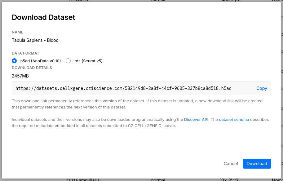
You can directly download the data clicking the button or copy the link and use the command line.

1wget https://datasets.cellxgene.cziscience.com/582149d8-2a8f-44cf-9605-337b8ca8d518.h5ad

To load the data we will use the scanpy package. First, we load the package with import scanpy as sc and then you can use the sc.read_h5ad function to load the data. The h5ad file is a hdf5 file with some modifications to store AnnData objects, see h5py for more details.

1# Specify the path to your .h5ad file
2file_path = "582149d8-2a8f-44cf-9605-337b8ca8d518.h5ad"
3
4# Read the .h5ad file into an AnnData object
5adata = sc.read_h5ad(file_path)

To inspect the data, we just need to print it.

1print(adata)

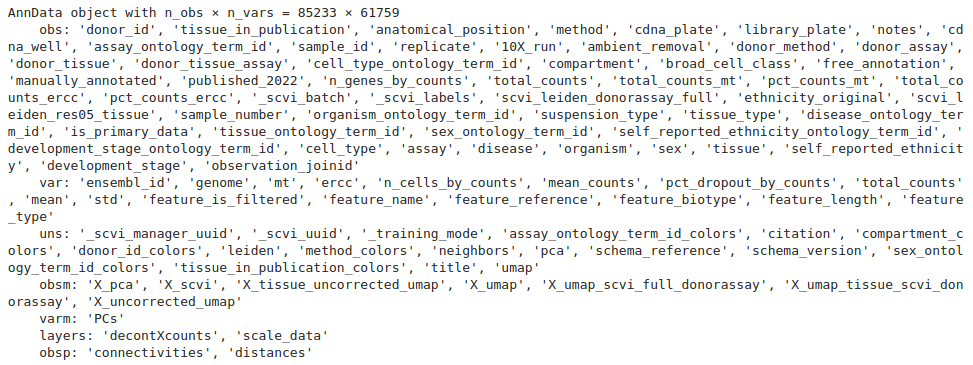
The first thing we see is that it is an AnnData object with 85233 observations and 61759 variables. The variables (columns) are the genes and the observations (rows) are the cells, it is important to keep this in mind when since most tools for single cell work the other way around, genes as rows and cells as columns.

AnnData object

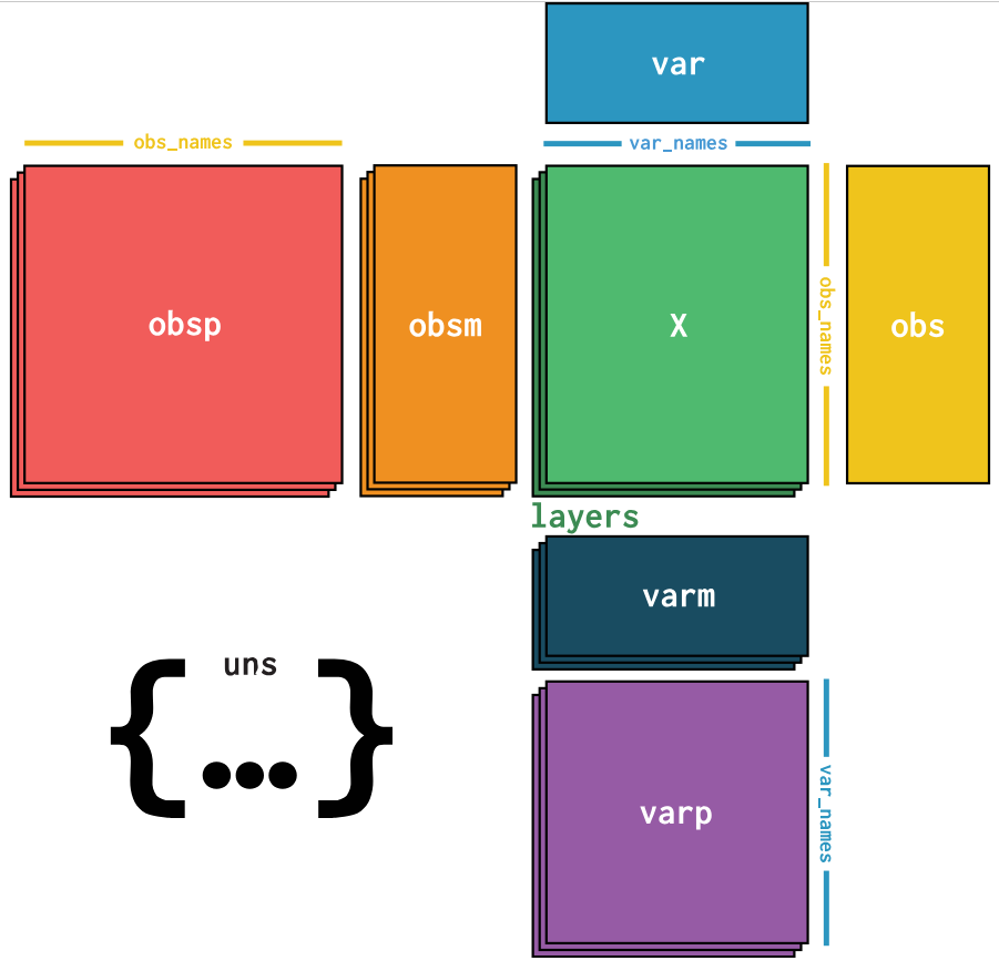
Since it is the core of the scanpy package, let's explore how AnnData (“Annotated Data”) objects work. anndata is a Python package for handling annotated data matrices and has this structure.

Expression data

The expression data is stored in the .X attribute, the row and column names are stored in the .obs and .var attributes respectively. The .obs attribute is a DataFrame with the cell names as index and the cell metadata as columns. The .var attribute is a DataFrame with the gene names as index and the gene metadata as columns.

Let's explore the expression data

1adata.X

It is a numpy object of float32 type. It is stored as a sparse matrix, this is because single cell data is usually very sparse, most cells will not express most genes. This is a good way to save memory and time when working with single cell data.

we can check the dimensions as follows:

1adata.X.shape

(85233, 61759)

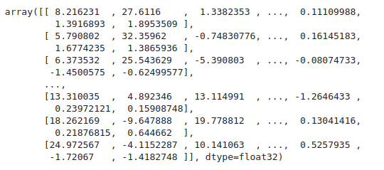
and the values of the matrix as follows:

1adata.to_df()

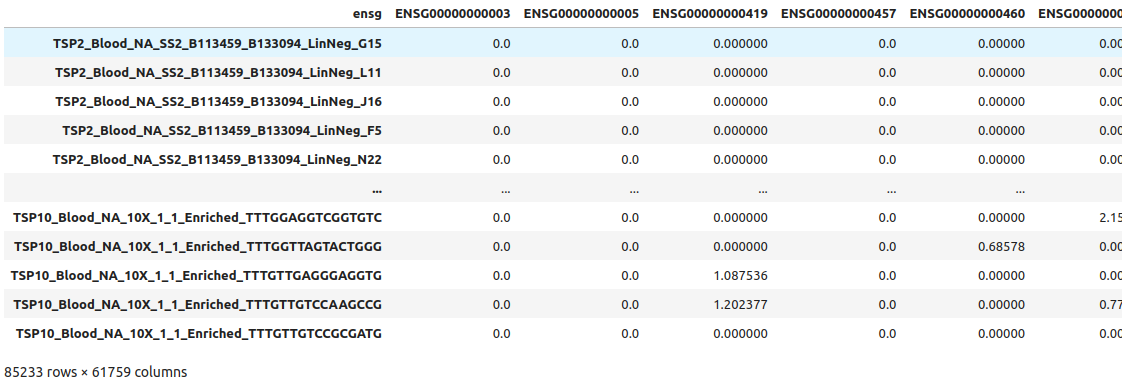
This is a pandas DataFrame with the expression data. We can visually confirm that columns are the genes and the rows are the cells.

Cell and gene metadata

The cell metadata is stored in the .obs attribute. This is a DataFrame with the cell names as index and the cell metadata as columns. Let's explore the cell metadata

1adata.obs

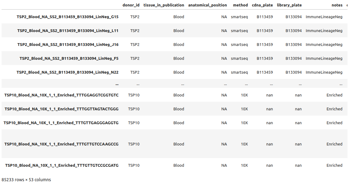
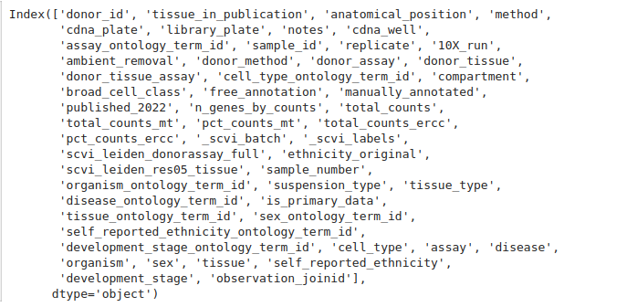
we see the different variables stored such as donor_id or notes for example. You can see the whole list of variables printing the adata object as before or with adata.obs.columns.

1adata.obs.columns

The gene metadata is stored in the .var attribute. This is a DataFrame with the gene names as index and the gene metadata as columns. It is accessed in the same way as the cell metadata.

1adata.var

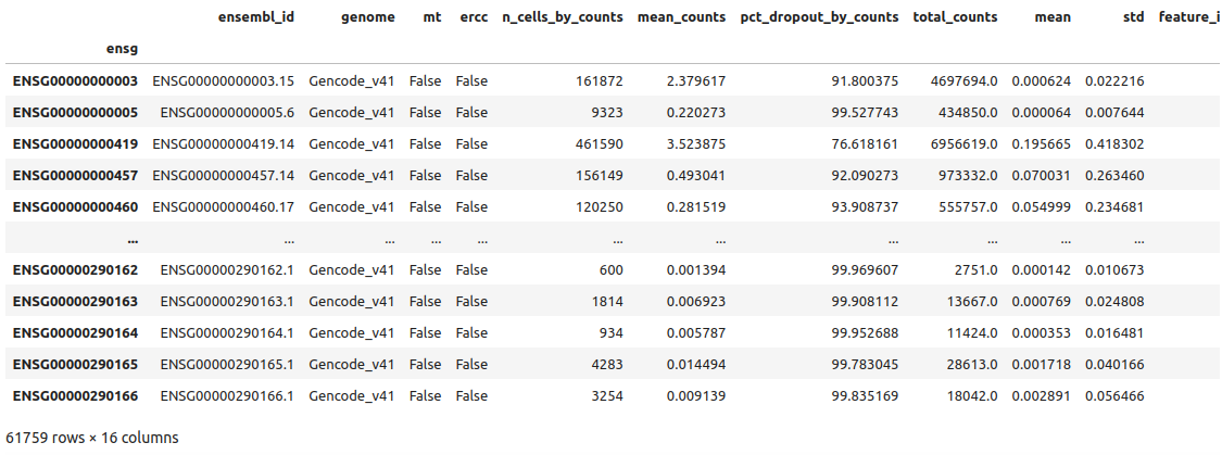
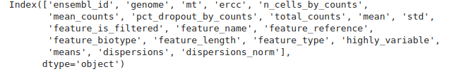
we see the different variables stored such as ensembl_id or feature_name for example. You can see the whole list of variables printing the adata object as before or with adata.var.columns.

1adata.var.columns

Matrix-level annotations

Matrix-level annotations for cells and genes are stored in the .obsm and .varm attributes, respectively. These are dictionaries that use keys to identify the different metadata-matrices.

For the cells, the .obsm usually stores the different cell embedding. Wwe can print the keys like this:

1adata.obsm.keys()

KeysView(AxisArrays with keys: X_pca, X_scvi, X_tissue_uncorrected_umap, X_umap, X_umap_scvi_full_donorassay, 
X_umap_tissue_scvi_donorassay, X_uncorrected_umap)

In this example we have different embeddings such as X_pca or X_umap. We can access the PCA data like this:

1adata.obsm["X_pca"]

Now we can check the gene-level annotations, note the different approach to access the data.

1adata.varm

AxisArrays with keys: PCs

These are the gene loadings for the PCA. Try to access the data using adata.varm["PCs"] and check the dimensions of the matrix (adata.varm['PCs'].shape).

Unstructured annotations

The .uns attribute is a dictionary where you can store any kind of information you want to keep with the data. This is useful to store information that is not cell or gene specific. For example, you can store the number of cells in the data set.

1adata.uns.keys()

dict_keys(['_scvi_manager_uuid', '_scvi_uuid', '_training_mode', 'assay_ontology_term_id_colors', 'citation', 
'compartment_colors', 'donor_id_colors', 'leiden', 'method_colors', 'neighbors', 'pca', 'schema_reference', 
'schema_version', 'sex_ontology_term_id_colors', 'tissue_in_publication_colors', 'title', 'umap', 'dendrogram_cell_type'])

In this example it contains very varied information ranging from the citation or the title of the data set to the colors used in the plots or the settings of some of the performed analyses (umap and leiden for example).

1adata.uns["umap"]

{'params': {'a': 0.583030019901822, 'b': 1.3341669931033755}}

Another interesting example is the pca key, which stores the variance of the components in addition to the parameters of the analysis.

1adata.uns["pca"]

{'params': {'use_highly_variable': False, 'zero_center': True},
 'variance': array([353.04341807, 306.68140918,  85.46049436,  46.43667367,
         27.63004892,  23.35384381,  21.28528965,  12.69999179,
         ...
         1.01804489,   0.97759633]),
 'variance_ratio': array([0.13888299, 0.12064474, 0.03361912, 0.01826762, 0.01086933,
        ...
        0.00042468, 0.00040952, 0.00040087, 0.00040049, 0.00038457])}

variance: Explained variance, equivalent to the eigenvalues of the covariance matrix.
variance_ratio: Explained variance ratio, i.e. percentage of total variance explain by each component.

obsp and varp

The .obsp and .varp attributes are used to store pairwise information between cells and genes, respectively. This is useful when you have pairwise information that you want to keep with the data. For example, you can store the distance between cells in the .obsp attribute or the correlation between genes in the .varp attribute.

Layers

The .layers attribute is a dictionary that stores additional data matrices. This is useful when you have multiple data matrices that you want to keep together. For example, you can store the raw data and the normalized data in the layers.

1adata.layers.keys()

KeysView(Layers with keys: decontXcounts, scale_data)

Save AnnData object

When you finish your analysis you can save the AnnData object to a h5ad file

1adata.write("blood_cells.h5ad")

Useful tips

Manual object creation

If you want to create an AnnData object from scratch you can use the AnnData class from the anndata package. You need to read the expression data, the cell and gene metadata and the matrix-level annotations separately and then create the object.

Prepare the data

 1# required packages
 2import numpy as np
 3import pandas as pd
 4import anndata as ad
 5import scipy.sparse as sp
 6import scanpy as sc
 7
 8# Load matrices
 9counts = pd.read_csv( "counts.csv", index_col=0)
10logcounts = pd.read_csv( "logcounts.csv", index_col=0)
11
12# Load metadata
13cell_metadata = pd.read_csv( "cell_metadata.csv", index_col=0)
14gene_metadata = pd.read_csv( "gene_metadata.csv", index_col=0)
15
16# Load matrix-level annotations: PCA, t-SNE, and UMAP embeddings
17pca = pd.read_csv( "PCA.csv", index_col=0)
18tsne = pd.read_csv( "TSNE.csv", index_col=0)
19umap = pd.read_csv( "UMAP.csv", index_col=0)

create annData object

 1# Create AnnData object
 2adata = ad.AnnData(
 3    X=sp.csr_matrix(logcounts.values),  # Sparse counts matrix
 4    obs=cell_metadata,                  # Cell metadata
 5    var=gene_metadata                   # Gene metadata
 6)
 7
 8# Add raw counts matrix to layers
 9adata.layers["counts"] = sp.csr_matrix(counts.values)   # Sparse counts matrix
10
11# Add PCA, t-SNE, and UMAP embeddings to obsm
12adata.obsm["X_pca"] = pca.values
13adata.obsm["X_tsne"] = tsne.values
14adata.obsm["X_umap"] = umap.values

Check the object

1adata

AnnData object with n_obs × n_vars = 3879 × 30157
    obs: 'cell', 'sample', 'label', 'batch'
    var: 'GeneID', 'GeneName', 'Chromosome'
    obsm: 'X_pca', 'X_tsne', 'X_umap'
    layers: 'counts'

Subsetting AnnData objects

These index values (gene and cell IDs) can be used to subset the AnnData, which provides a view of the AnnData object. This cab be useful to extract specific cell types or gene modules of interest. The approach is similar to subsetting a Pandas DataFrame. You can use values in the obs/var_names, boolean masks, or cell index integers.

1adata[["Cell_1", "Cell_10"], ["Gene_5", "Gene_1900"]]

View of AnnData object with n_obs × n_vars = 2 × 2

We can also subset based on cell metadata variables, in the blood cells example we can subset based on the donor_id or assay variable.

1set( adata.obs.assay ) # print the different assays

{"10x 3' v3", "10x 5' v2", 'Smart-seq2'}

1adata = adata[ adata.obs.assay == "10x 3' v3" ]
2adata.shape

(75461, 61759)

Note the cell (row) number has decreased from 85233 to 61759.

Big datasets

We can deal with large datasets by partially reading it into memory. Just select backed mode when reading the data.

1adata = ad.read('582149d8-2a8f-44cf-9605-337b8ca8d518.h5ad', backed='r')
2adata.isbacked

True

This option keeps an open file connection and only reads the data when needed

1adata.filename

PosixPath('582149d8-2a8f-44cf-9605-337b8ca8d518.h5ad')

so the connection must be closed at the end of the analysis.

1adata.file.close()

Take home messages

The AnnData object is the core data structure in scanpy.
Unlike SCE and Seurat, rows are cells’ barcodes and columns correspond to the gene IDs.
annData is designed to handle large datasets efficiently making Scanpy suitable for analyzing millions of cells, the example used is a clear example.

Next posts of this series will cover how to perform basic analyses with scanpy and how to integrate it with other tools. Stay tuned for similar posts on SingleCellExperiment and Seurat.