Single Cell PCA Deep Dive

Apr 16, 2025 · 7 min read · single cell code Bioconductor ·

Principal component analysis (PCA) is typical/obligated step of single cell data analysis. Using PCA allows us to reduce the number of dimensions in the data by 'compressing' the information of multiple genes into each principal component (PC). PCA reduces computations in downstream analysis, like clustering, and denoises the data.

Another advantage of PCA is that calculates the amount of variance from the original gene data explained by each PC. Thus, top PCs usually capture the dominant heterogeneity factors, i.e. relevant biological factors reflected in coexpression of multiple genes, while noise should be mainly found in last PCs since it affects genes randomly. All this suggests using top PCs in our downstream analyses to concentrating biological signals and reduce computations while removing noise.

And here we arrive to the topic of this post, how many PCs should be used?

Dataset

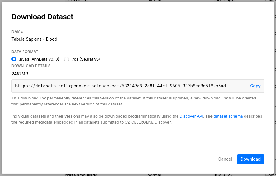
I will use the same dataset of blood cells from the cellxgene database that I used in my Scanpy, Seurat, and SCE posts.

1library(Seurat)
2rds.path <- '/media/alfonso/data/velocity_MGI/'
3rds.file <- file.path( rds.path, '582149d8-2a8f-44cf-9605-337b8ca8d518.rds' )
4seurat <- readRDS(rds.file)

This dataset contains cells from different donors and protocols, to keep it simple I will use cells from donor TSP1, and 10x 3' V3 technology. I will also remove cell types with less than 20 cells.

1library(dplyr)
2library(tidyr)
3library(tidylog)

1keep.cells <- seurat[[]] %>%
2  tibble::rownames_to_column( 'Cell' ) %>%
3  filter( assay == "10x 3' v3", donor_id == 'TSP1' ) %>%
4  group_by( cell_type ) %>%
5  mutate( tot = n() ) %>%
6  filter( tot >= 20 )

1## filter: removed 80,960 rows (95%), 4,273 rows remaining
2## group_by: one grouping variable (cell_type)
3## mutate (grouped): new variable 'tot' (integer) with 18 unique values and 0% NA
4## filter (grouped): removed 58 rows (1%), 4,215 rows remaining (removed 7 groups, 11 groups remaining)

1pbmc.filtered <- subset(seurat, cells = keep.cells$Cell)
2dim(pbmc.filtered)

1## [1] 61759  4215

Preprocessing

Convert Seurat object to SingleCellExperiment.

1pbmc.sce <- as.SingleCellExperiment(pbmc.filtered)
2pbmc.sce

 1## class: SingleCellExperiment 
 2## dim: 61759 4215 
 3## metadata(0):
 4## assays(2): counts logcounts
 5## rownames(61759): ENSG00000000003 ENSG00000000005 ... ENSG00000290165
 6##   ENSG00000290166
 7## rowData names(0):
 8## colnames(4215): TSP1_Blood_NA_10X3primev31_1_3_AAACCCAAGAATAGTC
 9##   TSP1_Blood_NA_10X3primev31_1_3_AAACCCAAGCAACAGC ...
10##   TSP1_Blood_NA_10X3primev31_1_2_TTTGGTTAGAGATCGC
11##   TSP1_Blood_NA_10X3primev31_1_2_TTTGGTTTCGCCAGTG
12## colData names(54): donor_id tissue_in_publication ...
13##   observation_joinid ident
14## reducedDimNames(7): PCA SCVI ... UMAP_TISSUE_SCVI_DONORASSAY
15##   UNCORRECTED_UMAP
16## mainExpName: RNA
17## altExpNames(0):

Keep the original dimensional reduction coordinates just in case, and remove unexpressed genes. I also save the original normalized counts.

1library(SingleCellExperiment)
2reducedDimNames(pbmc.sce) <- paste( reducedDimNames(pbmc.sce), 'Seurat', sep = '_' )
3pbmc.sce <- pbmc.sce[ rowSums( counts(pbmc.sce) ) != 0, ]
4assay( pbmc.sce, 'logcounts_Seurat' ) <- logcounts(pbmc.sce)
5logcounts(pbmc.sce) <- NULL
6pbmc.sce

 1## class: SingleCellExperiment 
 2## dim: 36413 4215 
 3## metadata(0):
 4## assays(2): counts logcounts_Seurat
 5## rownames(36413): ENSG00000000003 ENSG00000000419 ... ENSG00000290165
 6##   ENSG00000290166
 7## rowData names(0):
 8## colnames(4215): TSP1_Blood_NA_10X3primev31_1_3_AAACCCAAGAATAGTC
 9##   TSP1_Blood_NA_10X3primev31_1_3_AAACCCAAGCAACAGC ...
10##   TSP1_Blood_NA_10X3primev31_1_2_TTTGGTTAGAGATCGC
11##   TSP1_Blood_NA_10X3primev31_1_2_TTTGGTTTCGCCAGTG
12## colData names(54): donor_id tissue_in_publication ...
13##   observation_joinid ident
14## reducedDimNames(7): PCA_Seurat SCVI_Seurat ...
15##   UMAP_TISSUE_SCVI_DONORASSAY_Seurat UNCORRECTED_UMAP_Seurat
16## mainExpName: RNA
17## altExpNames(0):

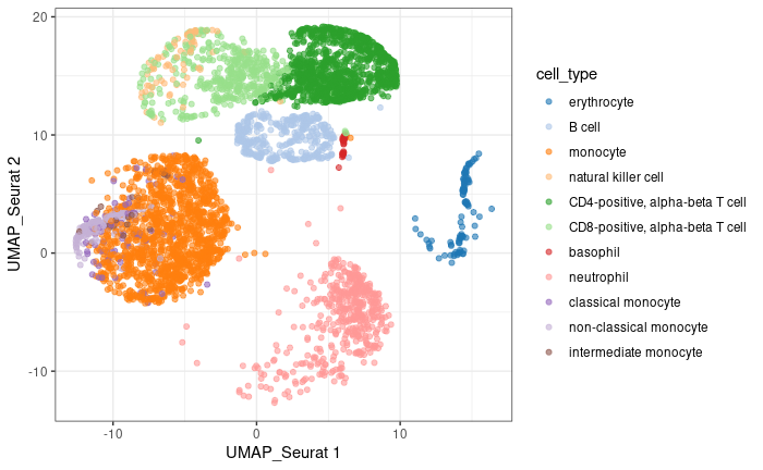
Check original UMAP

1library(scater)
2pbmc.sce$cell_type <- factor( pbmc.sce$cell_type )
3plotReducedDim( pbmc.sce, dimred = 'UMAP_Seurat', colour_by = 'cell_type' ) +
4  theme_bw()

Normalization by deconvolution

1library( scran )

1## Loading required package: scuttle

1pbmc.sce.clusters <- quickCluster(pbmc.sce)
2pbmc.sce <- computeSumFactors( pbmc.sce, 
3                               cluster=pbmc.sce.clusters, 
4                               min.mean=0.1
5                             )

1## Warning in .rescale_clusters(clust.profile, ref.col = ref.clust, min.mean = min.mean): inter-cluster rescaling factor for cluster 13 is not strictly positive,
2##   reverting to the ratio of average library sizes

1pbmc.sce <- logNormCounts( pbmc.sce )

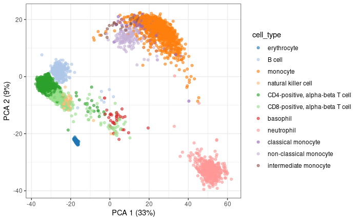
PCA

Calculate PCA using the 2000 top high variable genes

 1dec.pbmc.sce <- modelGeneVar( pbmc.sce )
 2top.HVGs <- getTopHVGs( dec.pbmc.sce, n=2000 )
 3
 4pbmc.sce <- runPCA( pbmc.sce, 
 5                    subset_row=top.HVGs, 
 6                    BPPARAM=BiocParallel::MulticoreParam(6)
 7                  )
 8
 9plotPCA( pbmc.sce, colour_by = 'cell_type' ) +
10  theme_bw()

Elbow point

A simple way of selecting the informative PCs is finding the elbow (point where the curve starts flatting out) in the scree plot (explained variance by PC).

1percent.var <- attr(reducedDim(pbmc.sce, 'PCA'), "percentVar")
2library(PCAtools)
3chosen.elbow <- findElbowPoint(percent.var)
4plot(percent.var, xlab="PC", ylab="Variance explained (%)")
5abline(v=chosen.elbow, col="red")

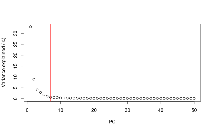
I will use t-SNE plots to evaluate the impact of using different number of PCs. Since the elbow point is at 7 PCs, I selected from 2 to 10 (2, 4, 7, 10), and then from 20 to 50 (in steps of 10)

 1for ( pcs in c( 2, 4, 7, 10, 10*(2:5) ) ){
 2  dimred.name <- paste0( 'PCA', pcs )
 3  reducedDim( pbmc.sce, dimred.name ) <- reducedDim( pbmc.sce, 'PCA' )[, 1:pcs]
 4  pbmc.sce <- runTSNE( pbmc.sce, dimred = dimred.name, 
 5                           BPPARAM=BiocParallel::MulticoreParam(8), 
 6                           name = paste0( 'TSNE.testPCs.', pcs )
 7  )
 8  g <- plotReducedDim( pbmc.sce, colour_by = 'cell_type', dimred = paste0( 'TSNE.testPCs.', pcs ) ) +
 9    theme_bw()
10  ggsave( plot = g, filename = paste0( 'TSNE.testPCs.', pcs, '.png' ), height = 5.86, width = 8.89 )
11}

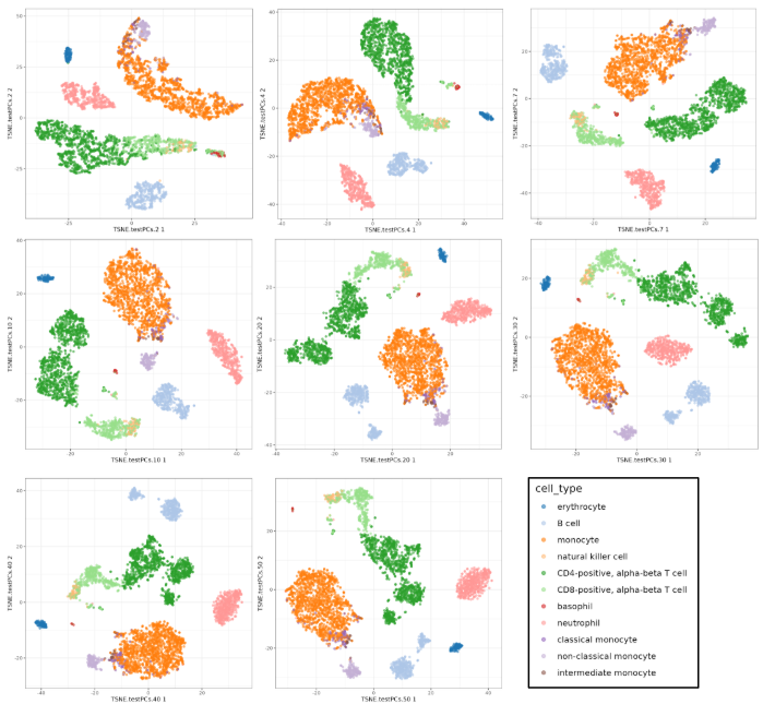
Conclusions

Using 7 PCs (elbow point) recapitulates well the original UMAP
Cell types are well separated with T cell subtypes appearing close but as separated groups
Similar results are found up to 10 PCs
Higher numbers of PCs subdivide main cell types in smaller groups, b cells and CD4+ T cells for example. It would be interesting to evaluate their biological relevance and the genes associated to the PCs driving these separations

Take away

It is advised to go higher in the number of selected PCs to avoid missing relevant biological information
Downstream analyses typically show small differences when a sufficient number of PCs are considered
Most guides and tutorials suggest using 10 - 50 PCs

Bonus: Animated Plots

Animated tSNE

 1library(gganimate)
 2
 3TSNE.plot.df <- lapply (grep( "TSNE.testPCs", reducedDimNames( pbmc.sce ), value = T ), function(redDim){
 4  pcs <- gsub( "TSNE.testPCs.", '', redDim )
 5  plot.df <- reducedDim( pbmc.sce, redDim ) %>%
 6    as.data.frame() %>%
 7    tibble::rownames_to_column( 'CELL' ) %>%
 8    mutate( PCs = as.integer(pcs) )
 9  
10}) %>%
11  bind_rows()
12
13
14cell.info.df <- colData(pbmc.sce) %>%
15  as.data.frame() %>%
16  tibble::rownames_to_column( 'CELL' ) %>%
17  select( CELL, type=cell_type )
18
19TSNE.plot.CELL.df <- full_join( TSNE.plot.df, cell.info.df, by = 'CELL' )
20
21TSNE.plot <- ggplot( TSNE.plot.CELL.df ) +
22  geom_point( aes(x=TSNE1, y = TSNE2, color = type, fill = type ), shape = 21, alpha = 0.5 ) +
23  theme_bw() +
24  theme( legend.position = 'none')
25
26TSNE.anim <- TSNE.plot + 
27  # transition_time( PCs )
28  transition_states(
29    PCs,
30    transition_length = 2,
31    state_length = 4
32  ) +
33  enter_fade() + 
34  exit_shrink() +
35  ease_aes('sine-in-out') +
36  labs(title = "PCs: {closest_state}")
37
38anim_save("TSNE.gif", TSNE.anim )

Animated explained variance

 1var.df <- data.frame( PC = 1:length(percent.var), variation = percent.var )
 2chosen.df <- var.df %>%
 3  mutate( step = PC ) %>%
 4  filter( step %in% TSNE.plot.CELL.df$PCs )
 5var.elbow.df <- var.df %>%
 6  mutate( text = 'Elbow', variation = max(variation) ) %>%
 7  filter( PC == chosen.elbow)
 8
 9scree.plot <- ggplot( var.df ) +
10  geom_point( aes(PC, variation ), shape = 21 ) +
11  geom_point( data=chosen.df, aes(PC, variation, group = interaction(PC, step) ), shape = 21, fill = 'blue' ) +
12  geom_vline( aes( xintercept = chosen.elbow ), color = 'red' ) +
13  geom_text( data =var.elbow.df, aes(PC, variation, label = text), color = 'red', hjust = -0.25 ) +
14  theme_bw() 
15
16scree.anim <- scree.plot +
17  transition_states(
18    states = step,
19    transition_length = 2,
20    state_length = 4
21  )  +
22  enter_fade() + 
23  exit_shrink() +
24  ease_aes('sine-in-out') +
25  labs(title = "PCs: {closest_state}")
26
27anim_save("PCs.gif", scree.anim )

Side by side animation https://github.com/thomasp85/gganimate/wiki/Animation-Composition https://stackoverflow.com/questions/49155038/how-to-save-frames-of-gif-created-using-gganimate-package

 1library( magick )
 2frames.path <- 'TSNE.frames'
 3dir.create( frames.path )
 4a_gif <- animate( TSNE.anim, width = 240, height = 240, nframes = 100, fps = 10,
 5                  renderer = file_renderer( dir = frames.path, prefix = "gganim_plot", overwrite = TRUE)
 6                )
 7
 8frames.path <- 'PCs.frames'
 9dir.create( frames.path )
10b_gif  <- animate( scree.anim, width = 240, height = 240, nframes = 100, fps = 10,
11                   renderer = file_renderer( dir = frames.path, prefix = "gganim_plot", overwrite = TRUE)
12                 )
13
14a_mgif <- image_read(a_gif)
15length( a_mgif )
16
17b_mgif <- image_read(b_gif)
18length( b_mgif )
19
20new_gif <- image_append(c(a_mgif[1], b_mgif[1]))
21for(i in 2:99){
22  combined <- image_append(c(a_mgif[i], b_mgif[i]))
23  new_gif <- c(new_gif, combined)
24}
25image_write(new_gif, path = "TSNE.PCs.gif", format = "gif")