Visium HD cell segmentation with Bin2Cell
Spatial transcriptomics reached a whole new level with the latest release from 10x Genomics, Visium HD. This state-of-the-art technology offers exceptional spatial resolution in transcriptomics, enabling researchers to map gene expression with unprecedented detail. From tumor microenvironments to intricate tissue architecture, Visium HD is transforming cellular biology experiments— pixel by pixel.
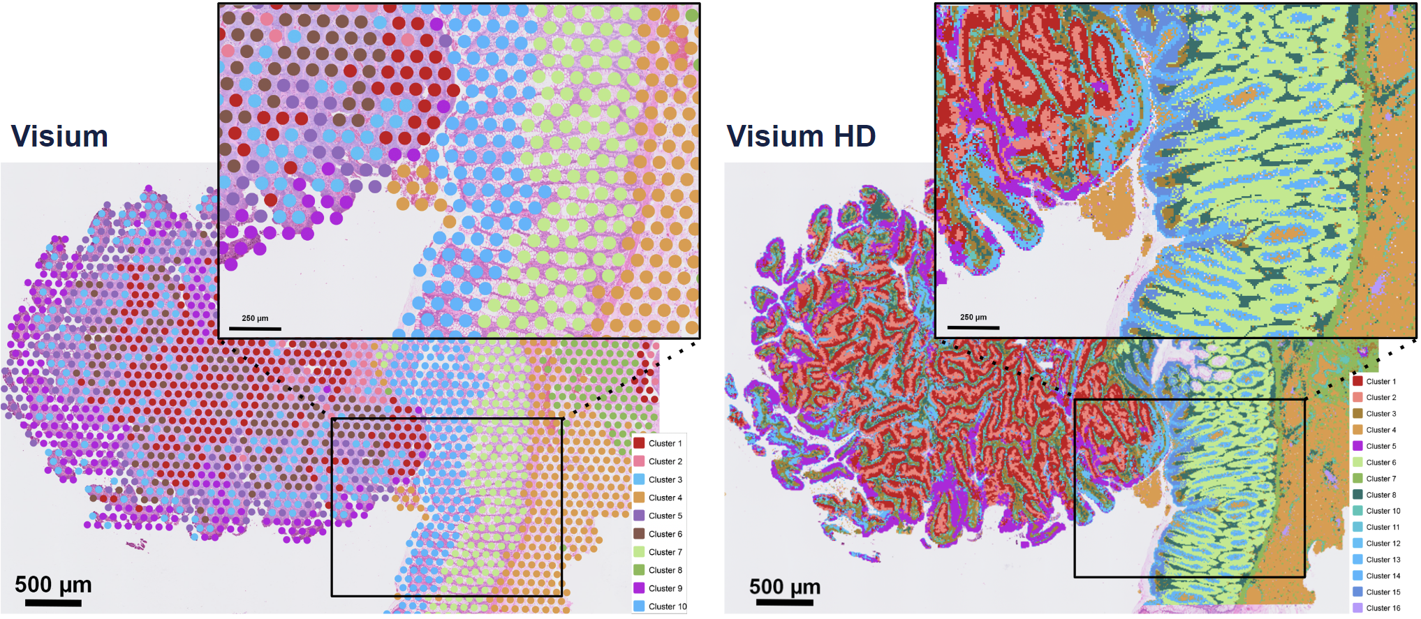
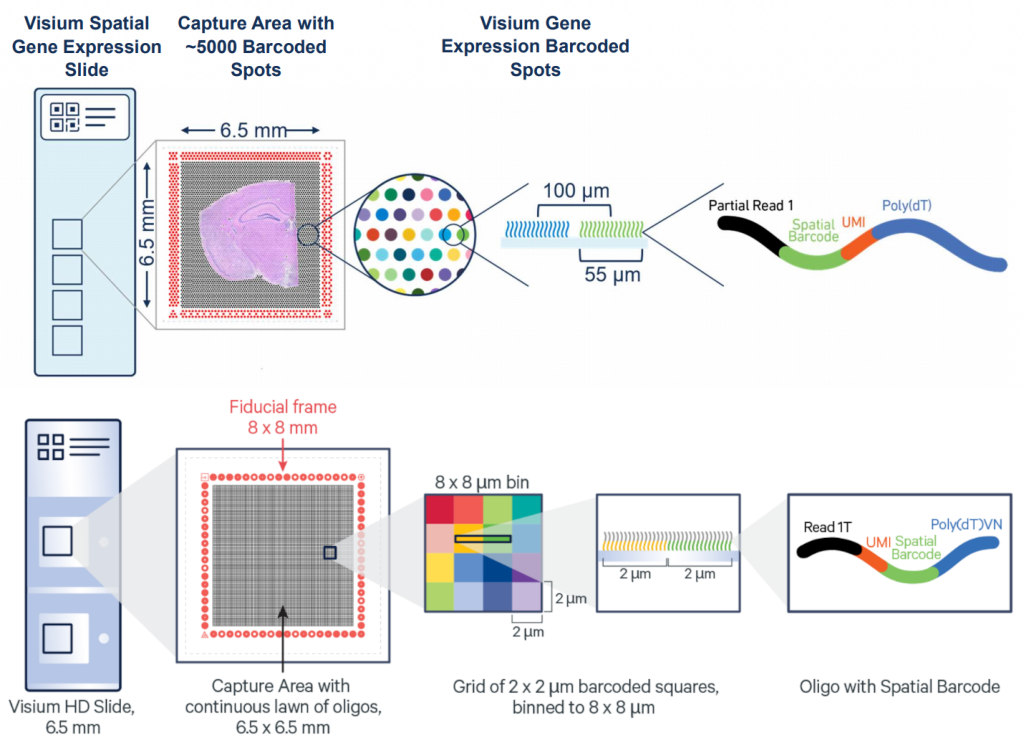
The key advantage of Visium HD over Visium is moving from discrete spots to a continuous lawn of oligonucleotides arrayed into millions of 2 x 2 µm barcoded squares that captures whole transcriptome expression.
Eventhough Visium HD provides extreme resolution, we still miss a key part to truly understand the biology of the system: single-cell individuality. Luckily for us, we can use segmentation techniques to reconstructs cells from the high resolution Visium HD data.
Following my previous post in VisiumHD nuclei segmentation today we explore bin2cell, a Python package to segment cells from Visium HD data that builds on the nuclei segmentation from the previous post.
You will need TensorFlow to perform this analysis. I run my code with jupyter notebook from a docker image as explained in my Using TensorFlow in 2025 post.
We start installing dependencies
1!apt-get update && apt-get install ffmpeg libsm6 libxext6 -y
and then the bin2cell package
1!pip install bin2cell
Load packages
1import matplotlib.pyplot as plt
2import scanpy as sc
3import numpy as np
4import os
5
6import bin2cell as b2c
Edit. Nov 2025
Space Ranger v4.0 (released in June 2025) now automatically performs nucleus-based cell segmentation for Visium HD and Visium HD 3' data if H&E images are provided.
Input data
As in the nuclei segmentation post, we will use the 10x Mouse Small Intestine (FFPE) dataset. Here we set the variables to find it.
1path = 'visium/' + "binned_outputs/square_002um/"
2source_image_path = 'visium/' + 'Visium_HD_Mouse_Small_Intestine_tissue_image.btf'
3spaceranger_image_path = 'visium/' + "spatial"
Load the data and inspect the annData object
1adata = b2c.read_visium(path,
2                        source_image_path = source_image_path,
3                        spaceranger_image_path = spaceranger_image_path
4                       )
5adata.var_names_make_unique()
6adata
anndata.py (1758): Variable names are not unique. To make them unique, call `.var_names_make_unique`.
anndata.py (1758): Variable names are not unique. To make them unique, call `.var_names_make_unique`.

AnnData object with n_obs × n_vars = 5479660 × 19059
    obs: 'in_tissue', 'array_row', 'array_col'
    var: 'gene_ids', 'feature_types', 'genome'
    uns: 'spatial'
    obsm: 'spatial'
Data cleaning
Here the code preprocesses the data to keep genes expressed in at least 3 spots and spots with at least 1 count.
1sc.pp.filter_genes(adata, min_cells=3)
2sc.pp.filter_cells(adata, min_counts=1)
3adata
AnnData object with n_obs × n_vars = 5367189 × 19000
    obs: 'in_tissue', 'array_row', 'array_col', 'n_counts'
    var: 'gene_ids', 'feature_types', 'genome', 'n_cells'
    uns: 'spatial'
    obsm: 'spatial'
Nuclei segmentation
Image preparation
As in the previous post, we need a custom H&E image to perform the segmentation with Stardist. The function b2c.scaled_he_image() creates this image and the resolution of the image is controlled by the mpp (microns per pixel) parameter. The StarDist models were trained on images with an mpp closer to 0.3, so we will use this value. However, it may need to be adjusted for specific experiments.
The b2c.scaled_he_image() function crops the image to an area around the actual spatial grid plus a default buffer of 150 pixels. The new coordinates are captured in .obsm["spatial_cropped_150_buffer"] and the new image can be used for plotting by providing basis="spatial_cropped_150_buffer" and img_key="0.5_mpp_150_buffer" to sc.pl.spatial().
1mpp = 0.3
2b2c.scaled_he_image(adata, mpp=mpp, save_path='visium/' + "stardist/he.tiff")
Cropped spatial coordinates key: spatial_cropped_150_buffer
Image key: 0.3_mpp_150_buffer
‘Striped’ effect correction
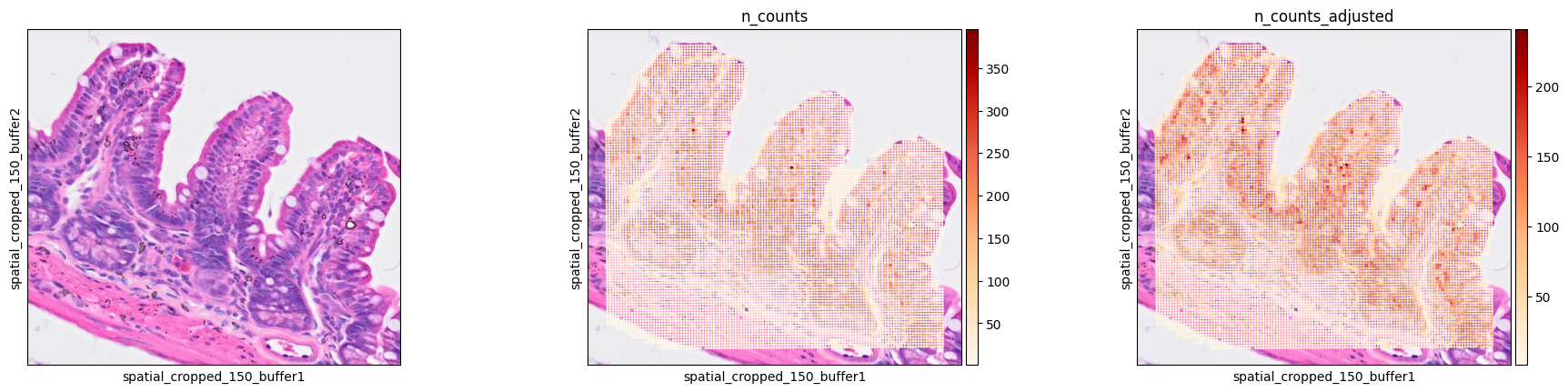
According to the authors, Visium HD 2um bins present variability in their width/height. When plotting total counts per spot, a striped pattern, where some rows/columns have fewer transcripts than others, appears.
The function b2c.destripe() is defined to correct for this. It identifies a quantile (default is 0.99) of total counts for each row and divides the counts of the spots in that row by that value. This procedure is then repeated for the columns and stored as .obs["n_counts_adjusted"]).
1b2c.destripe(adata)
_construct.py (163): Series.__getitem__ treating keys as positions is deprecated. In a future version, integer keys will always be treated as labels (consistent with DataFrame behavior). To access a value by position, use `ser.iloc[pos]`
To check the results, and compare with the previous post, we will use the same Region Of Interest (ROI) bbox=(12844,7700,13760,8664). However, we cannot use the image coordinates directly and, instead, we need to use the spatial coordinates to define the mask.
The following functions to get the spatial coordinates from the image coordinates, based on the min and max values for each axis and assuming they follow a linear relationship.
1def convert_row(pixel_coord):
2    b=60 # 60 = a * 0 + b
3    a=(3343-b)/21943 # 3343 = a * 21943 + b
4    return int(round(a*pixel_coord + b))
5
6def convert_col(pixel_coord):
7    b=131 # 131 = a * 0 + b
8    a=(3319-b)/23618 # 3319 = a * 23618 + b
9    return int(round(a*pixel_coord + b))
1bbox=(12844,7700,13760,8664)
2array_y_min=convert_row(bbox[1])
3array_y_max=convert_row(bbox[3])
4array_x_min=convert_col(bbox[0])
5array_x_max=convert_col(bbox[2])
6
7print("min x:\t{} --> {}\nmax x:\t{} --> {}\nmin y:\t{}  --> {}\nmax y:\t{}  --> {}\n".format(
8    bbox[0],array_x_min,bbox[2],array_x_max,bbox[1],array_y_min,bbox[3],array_y_max))
min x:	12844 --> 1865
max x:	13760 --> 1988
min y:	7700  --> 2191
max y:	8664  --> 2047
Here we define a mask to easily pull out this region of the object in the future, even with the linear transformation I had to correct the row coordinates a little bit to match the ROI in the previous post. Let me a comment if you have a better approach to get the spatial coordinates from the image coordinates.
1mask = ((adata.obs['array_row'] >= array_y_max+120) &
2        (adata.obs['array_row'] <= array_y_min+180) &
3        (adata.obs['array_col'] >= array_x_min) &
4        (adata.obs['array_col'] <= array_x_max)
5       )
6
7bdata = adata[mask]
Now we can check the results of the destripe function in our ROI.
1sc.pl.spatial(bdata, color=[None, "n_counts", "n_counts_adjusted"], color_map="OrRd",
2# sc.pl.spatial(adata, color=[None, "n_counts", "n_counts_adjusted"], color_map="OrRd", # use this one for full image. Takes long
3              img_key="0.3_mpp_150_buffer", basis="spatial_cropped_150_buffer")
931679955.py (8): Use `squidpy.pl.spatial_scatter` instead.
Nuclei prediction
In addition to the mpp parameter, the StarDist segmentation depends on this two parameters:
- prob_thresh: Probability threshold to remove low-confidence object predictions.
- nms_thresh: Overlap threshold to perform non-maximum suppression.
1b2c.stardist(image_path= 'visium/' + "stardist/he.tiff",
2             labels_npz_path= 'visium/' + "stardist/he.npz",
3             stardist_model="2D_versatile_he",
4             prob_thresh=0.01
5            )
2025-02-22 11:08:28.660918: E external/local_xla/xla/stream_executor/cuda/cuda_dnn.cc:9261] Unable to register cuDNN factory: Attempting to register factory for plugin cuDNN when one has already been registered
2025-02-22 11:08:28.662167: E external/local_xla/xla/stream_executor/cuda/cuda_fft.cc:607] Unable to register cuFFT factory: Attempting to register factory for plugin cuFFT when one has already been registered
2025-02-22 11:08:28.686936: E external/local_xla/xla/stream_executor/cuda/cuda_blas.cc:1515] Unable to register cuBLAS factory: Attempting to register factory for plugin cuBLAS when one has already been registered
2025-02-22 11:08:28.735251: I tensorflow/core/platform/cpu_feature_guard.cc:182] This TensorFlow binary is optimized to use available CPU instructions in performance-critical operations.
To enable the following instructions: AVX2 FMA, in other operations, rebuild TensorFlow with the appropriate compiler flags.
Found model '2D_versatile_he' for 'StarDist2D'.
Downloading data from https://github.com/stardist/stardist-models/releases/download/v0.1/python_2D_versatile_he.zip
5294730/5294730 [==============================] - 0s 0us/step
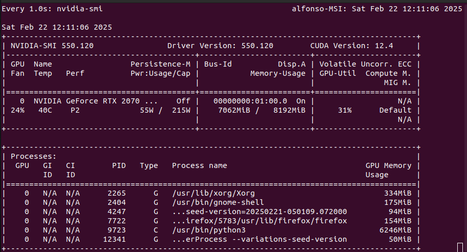
2025-02-22 11:09:25.310512: I tensorflow/core/common_runtime/gpu/gpu_device.cc:1929] Created device /job:localhost/replica:0/task:0/device:GPU:0 with 6123 MB memory: -> device: 0, name: NVIDIA GeForce RTX 2070 SUPER, pci bus id: 0000:01:00.0, compute capability: 7.5
Loading network weights from 'weights_best.h5'.
Loading thresholds from 'thresholds.json'.
Using default values: prob_thresh=0.692478, nms_thresh=0.3.
effective: block_size=(4096, 4096, 3), min_overlap=(128, 128, 0), context=(128, 128, 0)
2025-02-22 11:09:25.825480: I external/local_xla/xla/stream_executor/cuda/cuda_dnn.cc:454] Loaded cuDNN version 8906
2025-02-22 11:09:42.861200: W external/local_tsl/tsl/framework/cpu_allocator_impl.cc:83] Allocation of 536870912 exceeds 10% of free system memory.
100%|████████████████████████████████████████████████████████████████████| 36/36 [05:37<00:00, 9.37s/it]
Found 471627 objects
It complains again about TensorFlow (I removed the messages) but uses GPU and CPU resources.
We can now load the resulting cell calls into the object. The relevant parameters are:
- The labels generated in the previous step
- If the segmented image was based on array (GEX visualisation of the grid) or spatial (rescaled H&E image) coordinates
- The key that matches the image
- The mpp value used
1b2c.insert_labels(adata,
2                  labels_npz_path= 'visium/' + "stardist/he.npz",
3                  basis="spatial",
4                  spatial_key="spatial_cropped_150_buffer",
5                  mpp=mpp,
6                  labels_key="labels_he"
7                 )
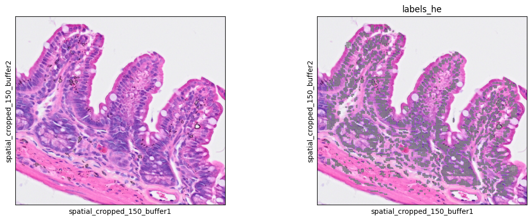
Now we visualize the results in the ROI.
1bdata = adata[mask]
2
3#the labels obs are integers, 0 means unassigned
4bdata = bdata[bdata.obs['labels_he']>0]
5bdata.obs['labels_he'] = bdata.obs['labels_he'].astype(str)
6
7sc.pl.spatial(bdata, color=[None, "labels_he"], img_key="0.3_mpp_150_buffer", basis="spatial_cropped_150_buffer", legend_loc='none')
2374757162.py (5): Trying to modify attribute `.obs` of view, initializing view as actual.
2374757162.py (7): Use `squidpy.pl.spatial_scatter` instead.
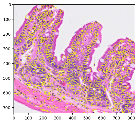
We can also see the segmentation results over the H&E image.
1#the label viewer wants a crop of the processed image
2#get the corresponding coordinates spanning the subset object
3crop = b2c.get_crop(bdata, basis="spatial", spatial_key="spatial_cropped_150_buffer", mpp=mpp)
4
5rendered = b2c.view_labels(image_path= 'visium/' + "stardist/he.tiff",
6                           labels_npz_path='visium/' + "stardist/he.npz",
7                           crop=crop
8                          )
9plt.imshow(rendered)
<matplotlib.image.AxesImage at 0x7f82ee7f2790>
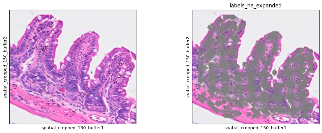
Nuclei expansion
Until now we have 'just' recreated the nuclei segmentation described in the previous post. Now it is time to expand the nuclei to get cell segmentation. The Bin2Cell package b2c.expand_labels function provides two methods:
- By default it expands each nuclei prediction adding bins up to
max_bin_distance(default 2) bins away from a labelled nucleus. - If
algorithm="volume_ratio"is set, each label gets a specific expansion distance derived based on the linear relationship between cell and nuclear volume. This relationship is controlled byvolume_ratio(default 4).
1b2c.expand_labels(adata,
2                  labels_key='labels_he',
3                  expanded_labels_key="labels_he_expanded"
4                 )
Now we check the expanded cells as follows
1bdata = adata[mask]
2
3#the labels obs are integers, 0 means unassigned
4bdata = bdata[bdata.obs['labels_he_expanded']>0]
5bdata.obs['labels_he_expanded'] = bdata.obs['labels_he_expanded'].astype(str)
6
7sc.pl.spatial(bdata, color=[None, "labels_he_expanded"], img_key="0.3_mpp_150_buffer", basis="spatial_cropped_150_buffer")
2208659422.py (5): Trying to modify attribute `.obs` of view, initializing view as actual.
2208659422.py (7): Use `squidpy.pl.spatial_scatter` instead.
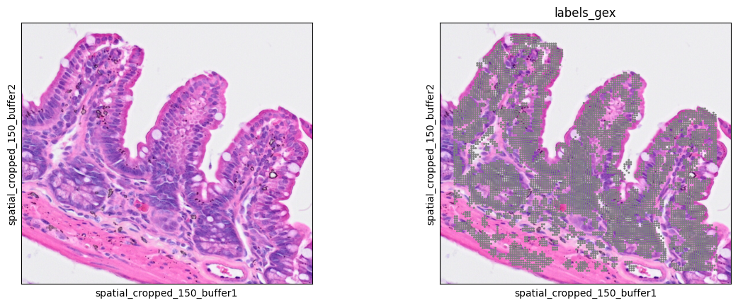
Label expansion
Since H&E segmentation may miss some nuclei. The Bin2Cell authors came up with an interesting approach, using total expression as fluorescence signal. They recommend using this approach as a secondary approach using its predictions only when H&E predictions are not present. Thus, the input image will be the total counts per bin, with a Gaussian filter with a sigma of 5 (measured in pixels) to smooth the signal a litle bit.
1b2c.grid_image(adata, "n_counts_adjusted", mpp=mpp, sigma=5, save_path= 'visium/' + "stardist/gex.tiff")
The segmentation is done using the StarDist's fluorescence model, and identifies cells instead of nuclei so the label expansion step is not necessary. The parameters are the same as before, but the model is different.
1b2c.stardist(image_path= 'visium/' + "stardist/gex.tiff",
2             labels_npz_path= 'visium/' + "stardist/gex.npz",
3             stardist_model="2D_versatile_fluo",
4             prob_thresh=0.05,
5             nms_thresh=0.5
6            )
Found model '2D_versatile_fluo' for 'StarDist2D'.
Downloading data from https://github.com/stardist/stardist-models/releases/download/v0.1/python_2D_versatile_fluo.zip
5320433/5320433 [==============================] - 0s 0us/step
Loading network weights from 'weights_best.h5'.
Loading thresholds from 'thresholds.json'.
Using default values: prob_thresh=0.479071, nms_thresh=0.3.
effective: block_size=(4096, 4096), min_overlap=(128, 128), context=(128, 128)


100%|████████████████████████████████████████████████████████████████████| 36/36 [08:33<00:00, 14.25s/it]


Found 290908 objects
Sometimes it fails to download the model, just re-run the command. The resulting predictions are loaded as before, using array instead of spatial as basis.
1b2c.insert_labels(adata,
2                  labels_npz_path='visium/'+"stardist/gex.npz",
3                  basis="array",
4                  mpp=mpp,
5                  labels_key="labels_gex"
6                 )
we check the new predictions in the ROI
1bdata = adata[mask]
2
3#the labels obs are integers, 0 means unassigned
4bdata = bdata[bdata.obs['labels_gex']>0]
5bdata.obs['labels_gex'] = bdata.obs['labels_gex'].astype(str)
6
7sc.pl.spatial(bdata, color=[None, "labels_gex"], img_key="0.3_mpp_150_buffer", basis="spatial_cropped_150_buffer")
3087949908.py (5): Trying to modify attribute `.obs` of view, initializing view as actual.
3087949908.py (7): Use `squidpy.pl.spatial_scatter` instead.
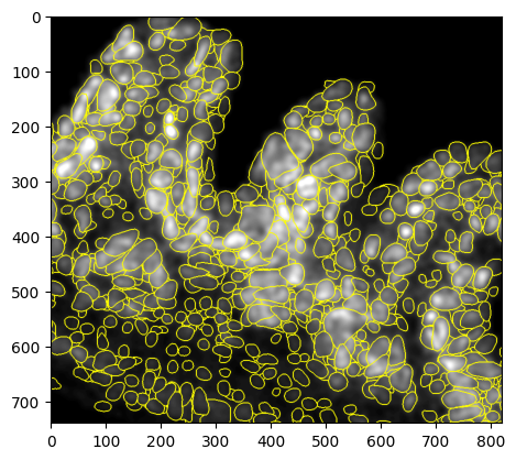
and the segmentation results on the pseudo-florescence input image.
 1#the label viewer wants a crop of the processed image
 2#get the corresponding coordinates spanning the subset object
 3crop = b2c.get_crop(bdata, basis="array", mpp=mpp)
 4
 5#GEX pops better with percentile normalisation performed
 6rendered = b2c.view_labels(image_path= 'visium/' + "stardist/gex.tiff",
 7                           labels_npz_path= 'visium/' + "stardist/gex.npz",
 8                           crop=crop,
 9                           stardist_normalize=True
10                          )
11plt.imshow(rendered)
<matplotlib.image.AxesImage at 0x7f82e91945d0>
Now we fill in the gaps in the H&E with GEX calls, as already said only using the GEX cells that do not overlap with any H&E labels.
1b2c.salvage_secondary_labels(adata,
2                             primary_label="labels_he_expanded",
3                             secondary_label="labels_gex",
4                             labels_key="labels_joint"
5                            )
Salvaged 22019 secondary labels
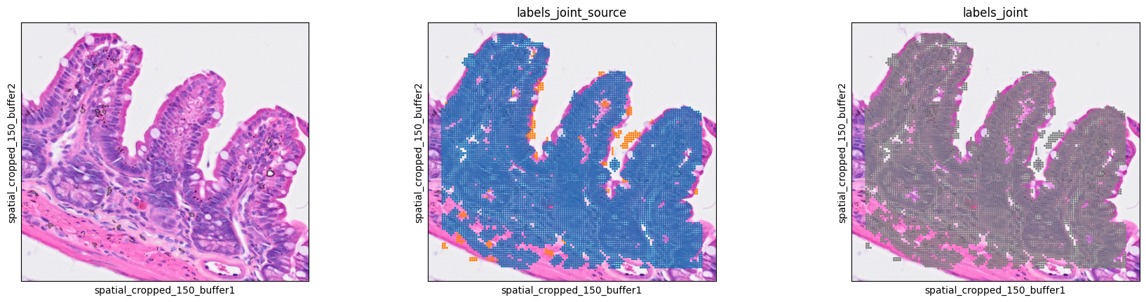
We can check the results as follows with the .obs["labels_joint_source"] key, which specifies whether any given label came from the primary or secondary labelling.
1bdata = adata[mask]
2
3#the labels obs are integers, 0 means unassigned
4bdata = bdata[bdata.obs['labels_joint']>0]
5bdata.obs['labels_joint'] = bdata.obs['labels_joint'].astype(str)
6
7sc.pl.spatial(bdata, color=[None, "labels_joint_source", "labels_joint"],
8              img_key="0.3_mpp_150_buffer", basis="spatial_cropped_150_buffer")
3308016099.py (5): Trying to modify attribute `.obs` of view, initializing view as actual.
3308016099.py (7): Use `squidpy.pl.spatial_scatter` instead.
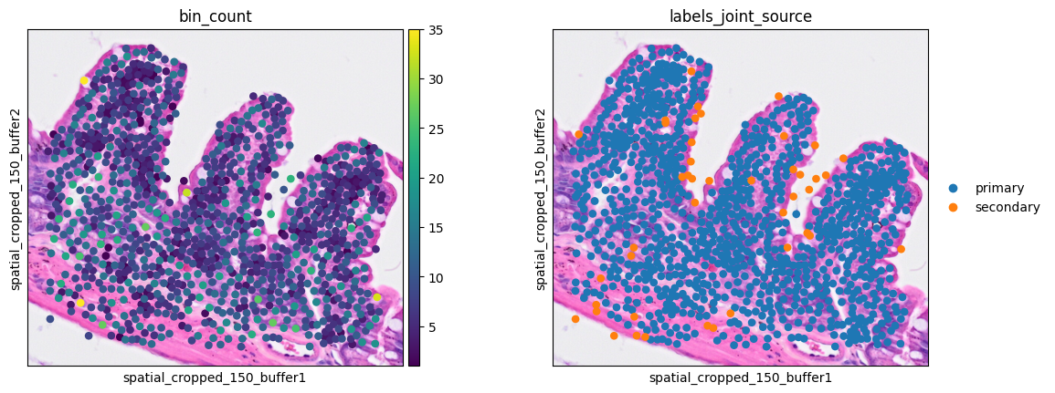
Cell bin aggregation
At this point, we can group the bins into cells and generate a new annData object.
1cdata = b2c.bin_to_cell(adata, labels_key="labels_joint", spatial_keys=["spatial", "spatial_cropped_150_buffer"])
In the new object contains the sum of gene expression of each cell assigned bins, with the mean of the array and spatial coordinates as the cell centroids. .obs["labels_joint_source"] is kept to provide information of the segmentation type. Let's check the cells in our ROI
1cell_mask = ((cdata.obs['array_row'] >= array_y_max+120) &
2             (cdata.obs['array_row'] <= array_y_min+180) &
3             (cdata.obs['array_col'] >= array_x_min) &
4             (cdata.obs['array_col'] <= array_x_max)
5            )
6
7ddata = cdata[cell_mask]
8sc.pl.spatial(ddata, color=[None, 'Lyz1'],
9              img_key="0.3_mpp_150_buffer", basis="spatial_cropped_150_buffer")
3308621866.py (2): Use `squidpy.pl.spatial_scatter` instead.
Clustering
To the downstream analysis, we start with the typical single cell RNAseq analysis pipeline, from normalization to clustering, using scanpy.
 1# Normalize total counts for each cell in the AnnData object
 2sc.pp.normalize_total(cdata, inplace=True)
 3
 4# Logarithmize the values in the AnnData object after normalization
 5sc.pp.log1p(cdata)
 6
 7# Identify highly variable genes in the dataset using the Seurat method
 8sc.pp.highly_variable_genes(cdata, flavor="seurat", n_top_genes=2000)
 9
10# Perform Principal Component Analysis (PCA) on the AnnData object
11sc.pp.pca(cdata)
12
13# Build a neighborhood graph based on PCA components
14sc.pp.neighbors(cdata)
15
16# Perform Leiden clustering on the neighborhood graph and store the results in 'clusters' column
17sc.tl.leiden(cdata, resolution=0.35, key_added="clusters")
Here we check the resulting object
1cdata
AnnData object with n_obs × n_vars = 480717 × 19000
    obs: 'object_id', 'bin_count', 'array_row', 'array_col', 'labels_joint_source', 'clusters'
    var: 'gene_ids', 'feature_types', 'genome', 'n_cells', 'highly_variable', 'means', 'dispersions', 'dispersions_norm'
    uns: 'spatial', 'log1p', 'hvg', 'pca', 'neighbors', 'clusters'
    obsm: 'spatial', 'spatial_cropped_150_buffer', 'X_pca'
    varm: 'PCs'
    obsp: 'distances', 'connectivities'
And get the number of cells per cluster
1cdata.obs['clusters'].value_counts()
clusters
0     101579
1      87628
2      72729
3      53883
4      31076
5      25481
6      14303
7      13436
8       8660
9       7120
10      6421
11      5168
12      4170
13      3560
14      3203
15      3169
16      3135
17      3017
18      2776
19      2485
20      2383
21      2350
22      2350
23      2125
24      1928
25      1796
26      1619
27      1599
28      1448
29      1419
30      1249
31      1228
32      1033
33       934
34       698
35       680
36       656
37       539
38       508
39       405
40       336
41       278
42        49
43        35
44        27
45        25
46        21
Name: count, dtype: int64
Let's see the clusters on the ROI for the shake of simplicity.
1ddata = cdata[cell_mask]
2sc.pl.spatial(ddata, color='clusters',
3              img_key="0.3_mpp_150_buffer", basis="spatial_cropped_150_buffer")
2477003661.py (2): Use `squidpy.pl.spatial_scatter` instead.
_utils.py (491): Trying to modify attribute `._uns` of view, initializing view as actual.
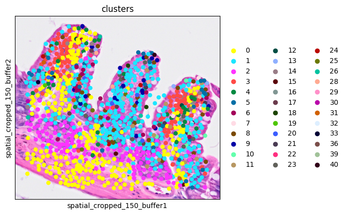
The clusters seem to correspond pretty well the tissue morphology.
Marker Genes
We will use the some specific cell type marker genes to evaluate the results.
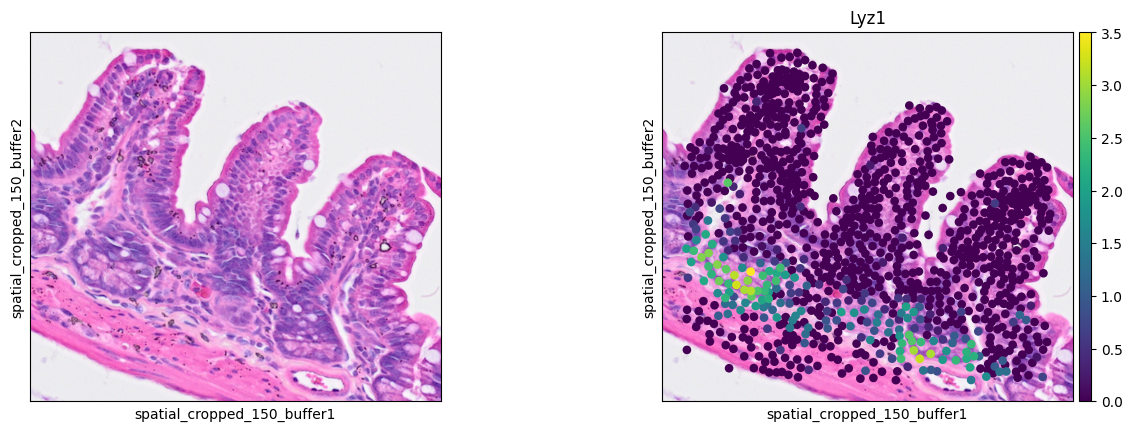
- Paneth cell: Lyz1
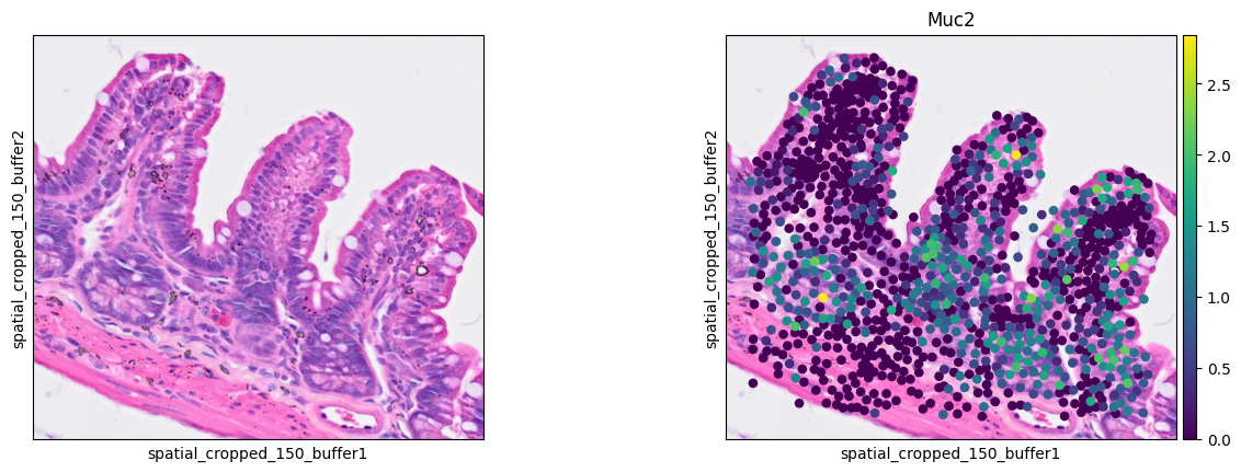
- Goblet cell: Muc2
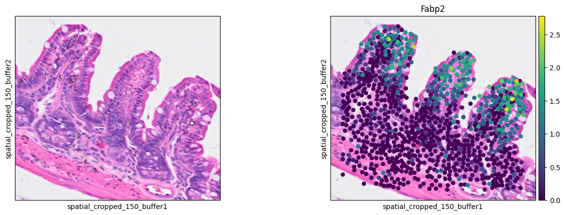
- Enterocyte cell: Fabp2
- Plasma cell: Jchain
This block defines a utility function, you can skip it if you want.
 1# coexpression summary
 2def calculate_summary(adata, gene_names):
 3    """
 4    Calculate the summary of the number of rows with both genes' expression == 0,
 5    each of the genes' expression == 0, and none of the genes' expression == 0.
 6
 7    Parameters:
 8    - adata: AnnData object
 9    - gene_names: list of two gene names (strings)
10
11    Returns:
12    - summary: dictionary containing the counts
13    """
14    gene1, gene2 = gene_names
15
16    # Get the indices of the genes
17    col1 = adata.var_names.get_loc(gene1)
18    col2 = adata.var_names.get_loc(gene2)
19
20    # Extract the expression data for the two genes
21    expr_data = adata.X[:, [col1, col2]].toarray()
22
23    both_zero = np.sum((expr_data[:, 0] == 0) & (expr_data[:, 1] == 0))
24    gene1_zero = np.sum((expr_data[:, 0] == 0) & (expr_data[:, 1] != 0))
25    gene2_zero = np.sum((expr_data[:, 0] != 0) & (expr_data[:, 1] == 0))
26    none_zero = np.sum((expr_data[:, 0] != 0) & (expr_data[:, 1] != 0))
27
28    summary = {
29        'both_zero': both_zero,
30        'gene1_zero': gene1_zero,
31        'gene2_zero': gene2_zero,
32        'none_zero': none_zero
33    }
34
35    return summary
Paneth cells
1ddata = cdata[cell_mask]
2sc.pl.spatial(ddata, color=[None, 'Lyz1'],
3              img_key="0.3_mpp_150_buffer", basis="spatial_cropped_150_buffer")
3308621866.py (2): Use `squidpy.pl.spatial_scatter` instead.
Goblet cells
1ddata = cdata[cell_mask]
2sc.pl.spatial(ddata, color=[None, 'Muc2'],
3              img_key="0.3_mpp_150_buffer", basis="spatial_cropped_150_buffer")
1464472417.py (2): Use `squidpy.pl.spatial_scatter` instead.
Enterocyte cells
1ddata = cdata[cell_mask]
2sc.pl.spatial(ddata, color=[None, 'Fabp2'],
3              img_key="0.3_mpp_150_buffer", basis="spatial_cropped_150_buffer")
1523107422.py (2): Use `squidpy.pl.spatial_scatter` instead.
Plasma cells
1ddata = cdata[cell_mask]
2sc.pl.spatial(ddata, color=[None, 'Jchain'],
3              img_key="0.3_mpp_150_buffer", basis="spatial_cropped_150_buffer")
3351794374.py (2): Use `squidpy.pl.spatial_scatter` instead.
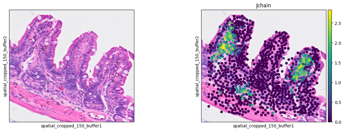
The marker analysis in the ROI seems quite good.
Segmentation analysis
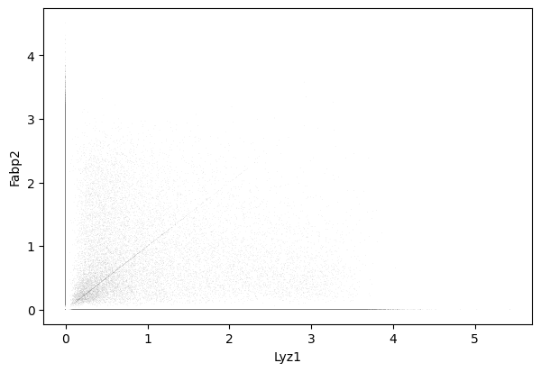
Segmentation analyses often face the issue of mixing cell types. We can evaluate it testing for cell type marker coexpression. We use scatter plots and the whole slide data.
Lyz1 and Fabp2
1sc.pl.scatter(cdata, x = 'Lyz1', y = 'Fabp2' )
 1gene_markers = ['Lyz1', 'Fabp2']
 2summary = calculate_summary(cdata, gene_markers )
 3total = sum(summary.values())
 4percentages = {key: (value / total) * 100 for key, value in summary.items()}
 5print( "Double negative: {:.2f}%\n{} positive: {:.2f}%\n{} positive: {:.2f}%\nDouble positive: {:.2f}%".format(
 6    percentages['both_zero'],
 7    gene_markers[1], percentages['gene1_zero'],
 8    gene_markers[0], percentages['gene2_zero'],
 9    percentages['none_zero']
10) )
Double negative: 49.23%
Fabp2 positive: 29.14%
Lyz1 positive: 18.64%
Double positive: 2.99%
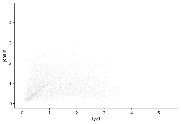
Lyz1 and Jchain
1sc.pl.scatter(cdata, x = 'Lyz1', y = 'Jchain' )
 1gene_markers = ['Lyz1', 'Jchain']
 2summary = calculate_summary(cdata, gene_markers )
 3total = sum(summary.values())
 4percentages = {key: (value / total) * 100 for key, value in summary.items()}
 5print( "Double negative: {:.2f}%\n{} positive: {:.2f}%\n{} positive: {:.2f}%\nDouble positive: {:.2f}%".format(
 6    percentages['both_zero'],
 7    gene_markers[1], percentages['gene1_zero'],
 8    gene_markers[0], percentages['gene2_zero'],
 9    percentages['none_zero']
10) )
Double negative: 64.37%
Jchain positive: 14.00%
Lyz1 positive: 18.22%
Double positive: 3.40%
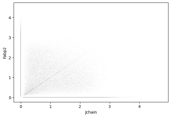
Jchain and Fabp2
1sc.pl.scatter(cdata, x = 'Jchain', y = 'Fabp2' )
 1gene_markers = ['Jchain', 'Fabp2']
 2summary = calculate_summary(cdata, gene_markers )
 3total = sum(summary.values())
 4percentages = {key: (value / total) * 100 for key, value in summary.items()}
 5print( "Double negative: {:.2f}%\n{} positive: {:.2f}%\n{} positive: {:.2f}%\nDouble positive: {:.2f}%".format(
 6    percentages['both_zero'],
 7    gene_markers[1], percentages['gene1_zero'],
 8    gene_markers[0], percentages['gene2_zero'],
 9    percentages['none_zero']
10) )
Double negative: 57.03%
Fabp2 positive: 25.56%
Jchain positive: 10.84%
Double positive: 6.57%
Cluster annotation
As a final step we can annotate (assign a cell type) our clusters. Again, we will check cell type marker expression using dot plots.
In dot plots, color intensity reflects gene expression levels, while dot size represents the proportion of cells expressing each gene across clusters. Larger, darker dots highlight genes with stronger and more widespread expression, facilitating the identification of distinct cell populations.
1# cd64: FCGR1. Intestinal macrophages markers https://pmc.ncbi.nlm.nih.gov/articles/PMC4451680/
2markers = { 'Paneth': 'Lyz1', 'Goblet': 'Muc2', 'Plasma Cell': 'Jchain', 'Enterocyte': 'Fabp2', 'T-cells': [ 'Cd3' + l for l in 'de' ], 'Macrophages': [ 'Fcgr1', 'Adgre1', 'Cd68' ] }
3p = sc.pl.dotplot(cdata, markers, groupby='clusters', dendrogram=True, return_fig=True)
4p.add_totals().style(dot_edge_color='black', dot_edge_lw=0.5).show()
WARNING: Groups are not reordered because the `groupby` categories and the `var_group_labels` are different.
categories: 0, 1, 2, etc.
var_group_labels: Paneth, Goblet, Plasma Cell, etc.
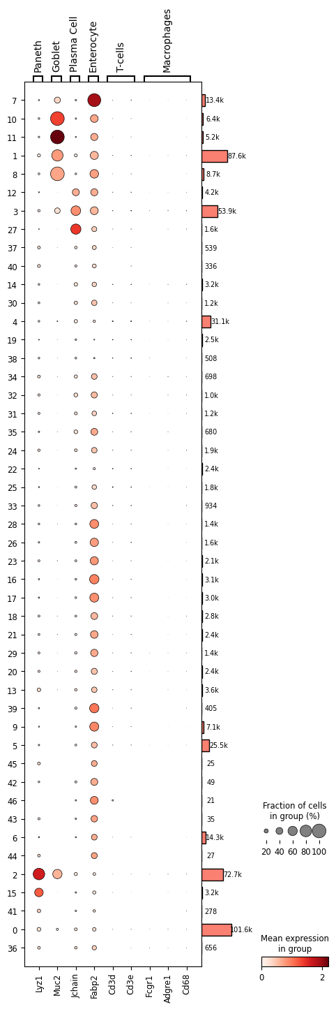
It seems clusters 2 and 15 corresponds to Paneth cells; clusters 1, 8, 10, 11 to Goblet cells; cluster 27 to Plasma cells; clusters 3 and 12 are difficult to differentiate between Plasma cells and Enterocytes. The remaining clusters would correspond to Enterocytes, with cluster 7 being the most evident, or remain unidentified (cluster 19 is a good example).
Again, apparently there are no T-cells or Macrophagues in this dataset. However, as discussed in the previous post these markers are used mainly for FACS cell selection and are often not very useful in transcriptomics approaches.
We would need to use multimodal approaches, combining protein and RNA detection or specific markers for these cell types at the transcriptomic level. Which markers would you use? Let's us know in the comments section below.
Take home messages
- Visium HD offers unparalleled spatial resolution providing a level of detail not seen before
- Nuclei segmentation is expanded to provide cell segmentation.
- Nuclei expanded labels are complemented with total expression prediction.
- Data can mislead, but your knowledge won’t—validate results with sanity checks, starting with marker expression.
This initial analysis did not find huge differences between the main results of the bin2cell cell segmentation and the previous nuclei segmentation. It makes sense since the startDist segmentation is a crucial step for the whole cell segmentation. A more detailed analysis would be needed to evaluate the differences between the two approaches.
Next posts of this series will use a different approach for cell segmentation and focus on providing a more in depth analysis of the obtained results. Leave your comments below.
Further reading
- Bin2Cell publication (Polański et al., 2024)
- Bin2Cell gihub
- Demo notebook
- StarDist segmentation relevant parameters guide, by Bin2Cell authors