Understanding Cellular Dynamics with RNA Velocity

Apr 28, 2025 · 7 min read · RNA velocity scVelo scanpy Pseudotime single cell RNAseq ·

Briefly speaking, RNA velocity is a single cell RNA-seq computational method to predict future gene expression states based on the ratio of spliced and unspliced mRNA transcripts.

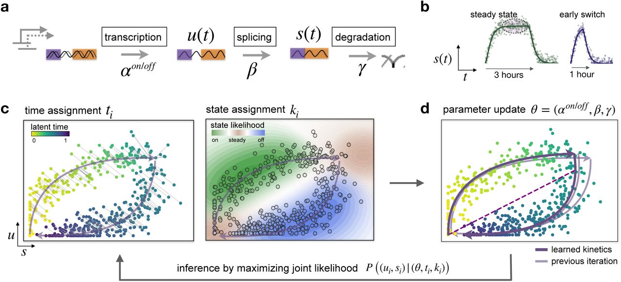
The original RNA velocity model, Velocyto, assumes a constant rate of transcription for each gene solving a system of linear differential equations. Later, scVelo was developed to improve the original implementation. It uses a dynamic model with a shared latent time across all cells and fits gene-specific transcription, splicing, and degradation parameters by likelihood-based expectation maximization

scVelo dynamical model solves the full splicing kinetics and generalizes to transient populations.

See the following animation by the scVelo team to better understand the relationship of the spliced vs. unspliced phase portrait with the abundance of pre-mRNA (unspliced) and mature mRNA (spliced)

For this post, I will use scVelo to estimate RNA velocity using the dynamical model of the same datasets used in my Pseudotime Trajectories with Slingshot post

Pancreas dataset

As in the Slingshot post, we use the dataset from Bastidas-Ponce et al. (2018) downloaded from scVelo github (https://github.com/theislab/scvelo_notebooks/tree/master/data/Pancreas/endocrinogenesis_day15.h5ad).

we start importing the required python packages

1import scanpy as sc
2import scvelo as scv

Next read the h5ad file as follows:

1adata = sc.read('endocrinogenesis_day15.h5ad')

and check the contents

1adata

AnnData object with n_obs × n_vars = 3696 × 27998
    obs: 'clusters_coarse', 'clusters', 'S_score', 'G2M_score'
    var: 'highly_variable_genes'
    uns: 'clusters_coarse_colors', 'clusters_colors', 'day_colors', 'neighbors', 'pca'
    obsm: 'X_pca', 'X_umap'
    layers: 'spliced', 'unspliced'
    obsp: 'distances', 'connectivities'

We start with standard preprocessing of the data

1scv.pp.filter_genes(adata, min_shared_counts=20)
2scv.pp.normalize_per_cell(adata)
3scv.pp.filter_genes_dispersion(adata, n_top_genes=2000)
4sc.pp.log1p(adata)

Filtered out 20801 genes that are detected 20 counts (shared).
Normalized count data: X, spliced, unspliced.
Extracted 2000 highly variable genes.

Next calculate first and second order moments

1scv.pp.moments(adata, n_pcs=30, n_neighbors=30)

computing neighbors
    finished (0:00:05) --> added 
    'distances' and 'connectivities', weighted adjacency matrices (adata.obsp)
computing moments based on connectivities
    finished (0:00:00) --> added 
    'Ms' and 'Mu', moments of un/spliced abundances (adata.layers)

We now run the dynamical model to infer the complete transcriptional dynamics underlying splicing kinetics. This is achieved using a likelihood-based expectation-maximization framework, which iteratively estimates both the reaction rate parameters and latent cell-specific variables. These are the transcriptional state and each cell’s internal latent time. The goal is to reconstruct the unspliced/spliced phase trajectory for each gene.

1scv.tl.recover_dynamics(adata)

recovering dynamics (using 1/8 cores)
WARNING: Unable to create progress bar. Consider installing `tqdm` as `pip install tqdm` and `ipywidgets` as `pip install ipywidgets`,
or disable the progress bar using `show_progress_bar=False`.
    finished (0:06:24) --> added 
    'fit_pars', fitted parameters for splicing dynamics (adata.var)

Now we can estimate RNA velocity using the dynamical model, which are stored in adata.layers.

1scv.tl.velocity(adata, mode='dynamical')

computing velocities
    finished (0:00:02) --> added 
    'velocity', velocity vectors for each individual cell (adata.layers)

The combination of velocities across genes can then be used to estimate the future state of an individual cell. In order to project the velocities into a lower-dimensional embedding, transition probabilities of cell-to-cell transitions are estimated. That is, for each velocity vector we find the likely cell transitions that are accordance with that direction. The transition probabilities are computed using cosine correlation between the potential cell-to-cell transitions and the velocity vector, and are stored in a matrix denoted as velocity graph.
— scVelo tutorial

1scv.tl.velocity_graph(adata)

computing velocity graph (using 1/8 cores)
    finished (0:00:05) --> added 
    'velocity_graph', sparse matrix with cosine correlations (adata.uns)

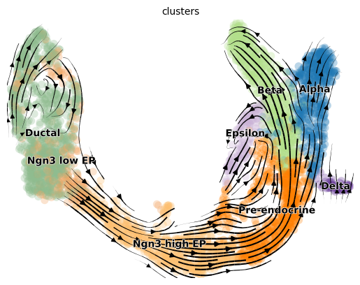
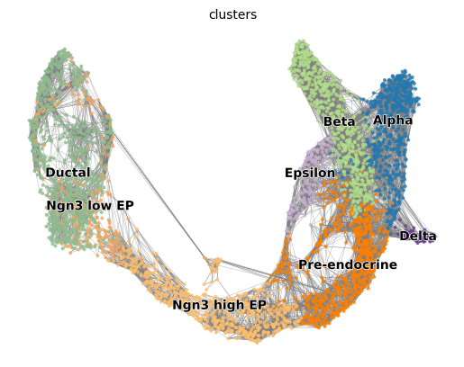
Project the velocities onto UMAP as streamlines

1scv.pl.velocity_embedding_stream(adata, basis='umap')

computing velocity embedding
    finished (0:00:00) --> added
    'velocity_umap', embedded velocity vectors (adata.obsm)

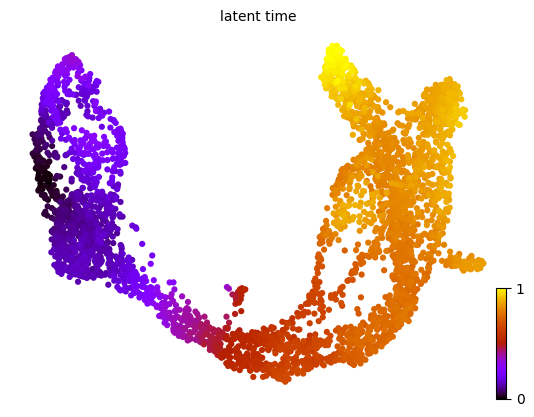
Latent time

The dynamical model infers the latent time of the underlying cellular processes, capturing each cell’s internal clock. This latent time reflects an estimate of the actual progression experienced by cells during differentiation, derived solely from the transcriptomic data.

1scv.tl.latent_time(adata)
2scv.pl.scatter(adata, color='latent_time', color_map='gnuplot', size=80)

computing terminal states
    identified 2 regions of root cells and 1 region of end points .
    finished (0:00:00) --> added
    'root_cells', root cells of Markov diffusion process (adata.obs)
    'end_points', end points of Markov diffusion process (adata.obs)
computing latent time using root_cells as prior
    finished (0:00:00) --> added 
    'latent_time', shared time (adata.obs)

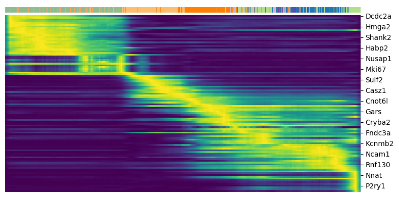
Driver genes are selected as those with high likelihoods in the dynamic model. The likelihood of a gene is defined as the probability of observing the data given the model parameters. The higher the likelihood, the better the model fits the data. Genes with high likelihoods are more likely to be involved in the underlying biological process.

1top_genes = adata.var['fit_likelihood'].sort_values(ascending=False).index[:100]
2scv.pl.heatmap(adata, var_names=top_genes, sortby='latent_time', col_color='clusters', n_convolve=100)

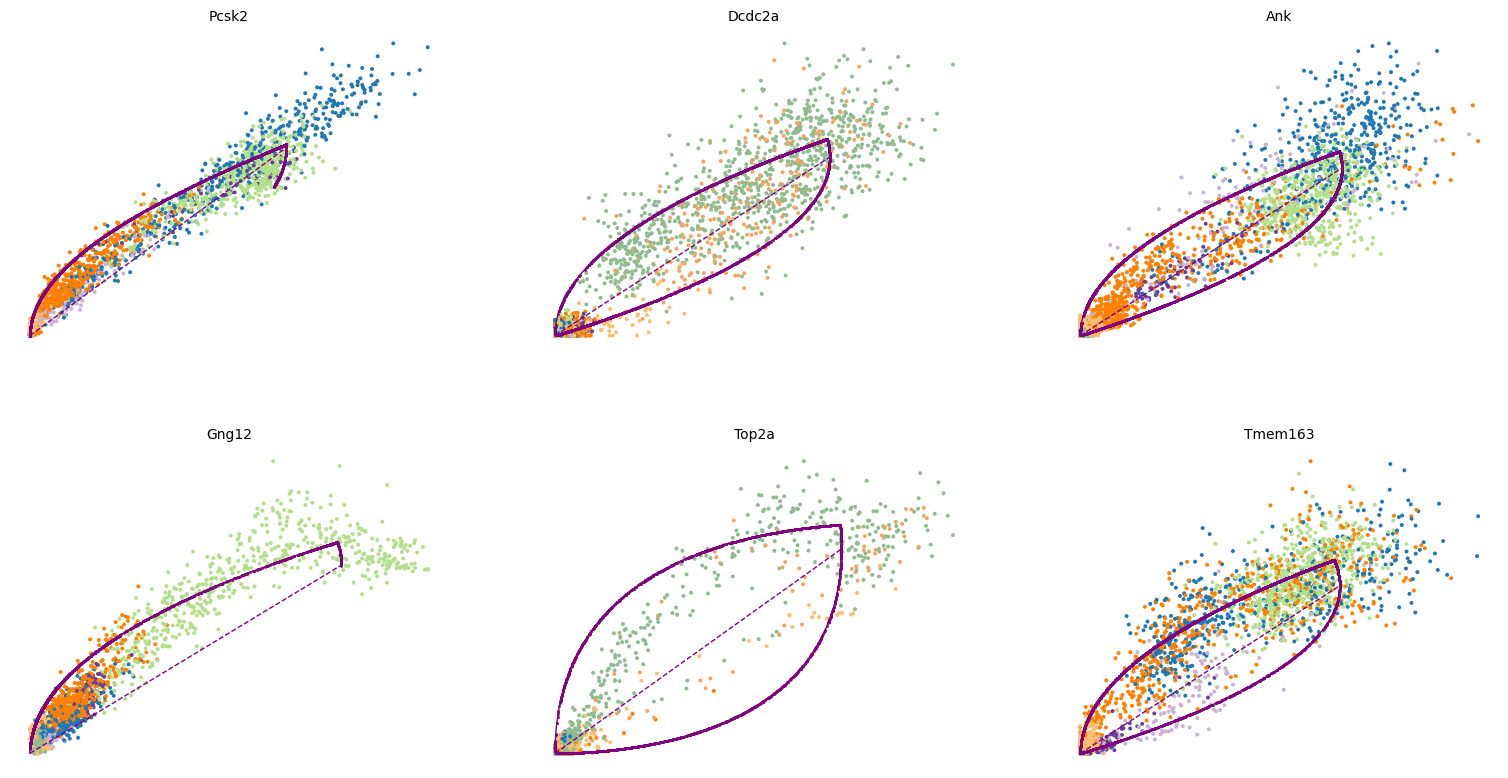
Here we check a few of the top likelihood genes using phase portraits.

1top_genes = adata.var['fit_likelihood'].sort_values(ascending=False).index
2scv.pl.scatter(adata, basis=top_genes[:6], ncols=3, frameon=False)

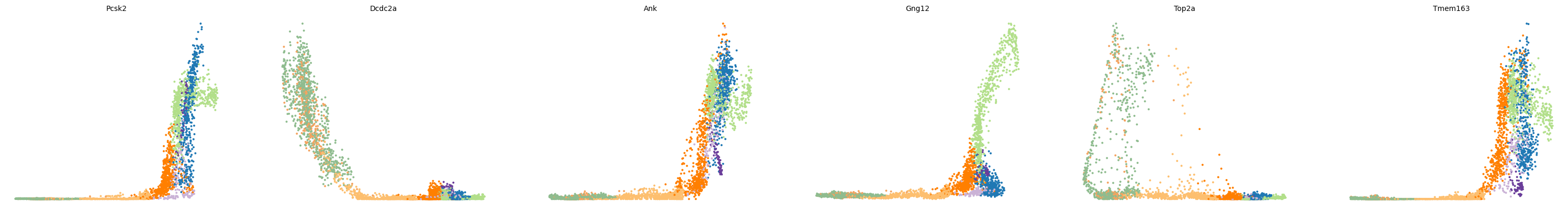
and their expression along the calculated latent time

1scv.pl.scatter(adata, x='latent_time', y=top_genes.values[:6], frameon=False)

We can plot the velocity graph to visualize all velocity-inferred cell connections/transitions.

1scv.pl.velocity_graph(adata, threshold=.1)

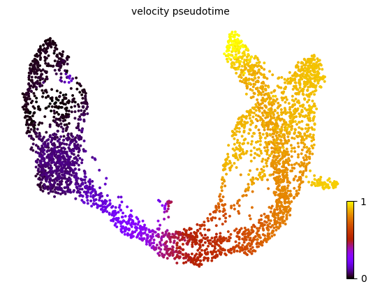
based on the velocity graph, a velocity pseudotime can be computed.

1scv.tl.velocity_pseudotime(adata)
2scv.pl.scatter(adata, color='velocity_pseudotime', cmap='gnuplot')

save the object

1adata.write('pancreas.withVelocity.h5ad')

Spermatogenesis Data

Again, we use the same dataset as in the Slingshot post from Hermann et al. (2018), downloaded from the scRNAseq package and coverted to h5ad format using the zellkonverter package in R as follows

1library(zellkonverter)
2writeH5AD(sce.sling, file = 'spermatogenesis.slingshot.h5ad', verbose = TRUE)

So we can read the h5ad file as follows in python

1adata = sc.read('spermatogenesis.slingshot.h5ad')

and check the contents

1adata

AnnData object with n_obs × n_vars = 1816 × 29826
    obs: 'celltype', 'sum', 'detected', 'subsets_Mt_sum', 'subsets_Mt_detected', 'subsets_Mt_percent', 'total', 'sizeFactor', 'slingPseudotime_1'
    uns: '.colData', 'X_name'
    obsm: 'PCA', 'UMAP', 'UMAP_3D'
    layers: 'spliced', 'unspliced'

the pl.embedding function expects a numpy array but the conversor generated a pandas df

1adata.obsm["UMAP"]

	UMAP1	UMAP2
CCCATACTCCGAAGAG	8.908866	5.790795
AATCCAGTCATCTGCC	9.038168	5.535748
GACTGCGGTTTGACTG	9.124887	5.500014
ACACCAATCTTCGGTC	9.187134	5.613092
TGACAACAGGACAGAA	2.905884	-6.314294
...	...	...
TGCGTGGGTATATGGA	-9.742685	7.182144
TTAACTCAGTTGAGAT	6.960753	5.540197
TAGCCGGAGGAATCGC	-9.991141	6.813681
TCGCGTTCAAGAGTCG	-1.258456	4.865719
CACCTTGCAGATCGGA	-1.269776	4.853017

1816 rows × 2 columns

1print(type(adata.obsm['UMAP']))

<class 'pandas.core.frame.DataFrame'>

so it must be converted to a numpy array

1adata.obsm['UMAP'] = adata.obsm['UMAP'].to_numpy()

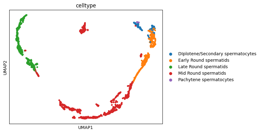
Now we can plot the UMAP embedding

1sc.pl.embedding(adata, basis = 'UMAP', color = 'celltype' )

Since the data was already preprocessed in the Slingshot post we can directly calculate the first and second order moments

1scv.pp.moments(adata, n_pcs=30, n_neighbors=30)

computing neighbors
    finished (0:00:00) --> added 
    'distances' and 'connectivities', weighted adjacency matrices (adata.obsp)
computing moments based on connectivities
    finished (0:00:02) --> added 
    'Ms' and 'Mu', moments of un/spliced abundances (adata.layers)

it recomputes PCA to perform the moments calculations since it was not stored with the expected key.

1adata

AnnData object with n_obs × n_vars = 1816 × 29826
    obs: 'celltype', 'sum', 'detected', 'subsets_Mt_sum', 'subsets_Mt_detected', 'subsets_Mt_percent', 'total', 'sizeFactor', 'slingPseudotime_1'
    uns: '.colData', 'X_name', 'celltype_colors', 'pca', 'neighbors'
    obsm: 'PCA', 'UMAP', 'UMAP_3D', 'X_pca'
    varm: 'PCs'
    layers: 'spliced', 'unspliced', 'Ms', 'Mu'
    obsp: 'distances', 'connectivities'

run dynamical model

1scv.tl.recover_dynamics(adata)

recovering dynamics (using 1/8 cores)
    finished (0:24:11) --> added 
    'fit_pars', fitted parameters for splicing dynamics (adata.var)

and Estimate RNA velocity

1scv.tl.velocity(adata, mode='dynamical')
2scv.tl.velocity_graph(adata)

computing velocities
    finished (0:00:08) --> added 
    'velocity', velocity vectors for each individual cell (adata.layers)
computing velocity graph (using 1/8 cores)
    finished (0:00:14) --> added 
    'velocity_graph', sparse matrix with cosine correlations (adata.uns)

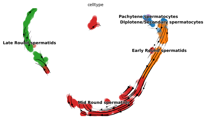
project the velocities onto UMAP as streamlines

1scv.pl.velocity_embedding_stream(adata, basis='UMAP', color = 'celltype' )

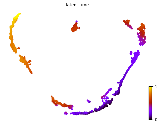
calculate latent time

1scv.tl.latent_time(adata)
2scv.pl.scatter(adata, basis='UMAP', color='latent_time', color_map='gnuplot', size=80)

computing terminal states
    identified 1 region of root cells and 1 region of end points .
    finished (0:00:00) --> added
    'root_cells', root cells of Markov diffusion process (adata.obs)
    'end_points', end points of Markov diffusion process (adata.obs)
computing latent time using root_cells as prior
    finished (0:00:02) --> added 
    'latent_time', shared time (adata.obs)

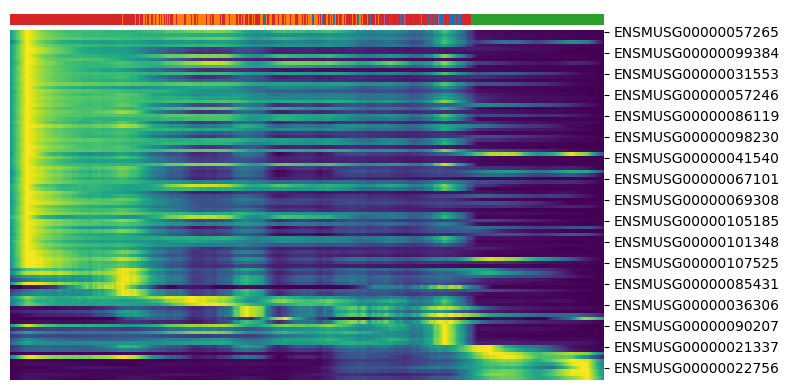
get the driver genes and plot the heatmap

1top_genes = adata.var['fit_likelihood'].sort_values(ascending=False).index[:100]
2scv.pl.heatmap(adata, var_names=top_genes, sortby='latent_time', col_color='celltype', n_convolve=100)

/home/alfonso/.virtualenvs/scvelo/lib/python3.10/site-packages/scvelo/plotting/utils.py:68: DeprecationWarning: is_categorical_dtype is deprecated and will be removed in a future version. Use isinstance(dtype, pd.CategoricalDtype) instead
  return isinstance(c, str) and c in data.obs.keys() and cat(data.obs[c])

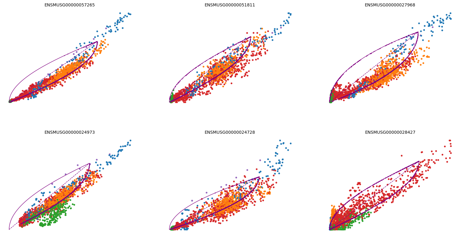
and scatter plots

1top_genes = adata.var['fit_likelihood'].sort_values(ascending=False).index
2scv.pl.scatter(adata, basis=top_genes[:6], ncols=3, frameon=False, color='celltype')

1scv.pl.scatter(adata, x='latent_time', y=top_genes.values[:6], frameon=False, color='celltype')

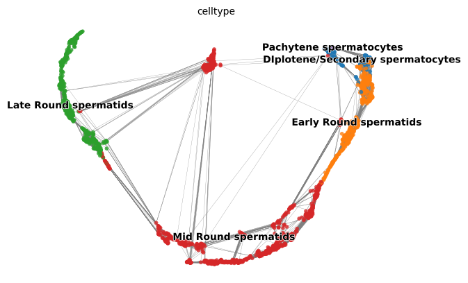
and Estimate RNA velocity

1scv.pl.velocity_graph(adata, basis = 'UMAP', threshold=.1, color='celltype')

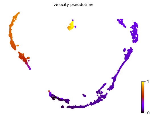
1scv.tl.velocity_pseudotime(adata)
2scv.pl.scatter(adata, basis = 'UMAP', color='velocity_pseudotime', cmap='gnuplot')

save the object as follows

1adata.write('spermatogenesis.withVelocity.h5ad')

Conclusions

The dynamic model of scVelo is able to decipher distinct kinetic behaviors (e.g., transcriptional activity, splicing rates, differentiation timing) to describe the underlying differentiation processes.
Selecting genes with high likelihood successfully identifies dynamically changing genes

Take away

scVelo calculates two differential times: latent time and velocity pseudotime
- Latent time is calculated directly from the count values.
- Velocity pseudotime is a diffusion pseudotime computed based on the scVelo velocity graph and root cells obtained from the velocity-inferred transition matrix. You can see it as being analogous to the pseudotime calculated by Slingshot.
According to the authors, latent time truly captures the underlying differentiation time.