Single Cell Dimensional Reduction: t-SNE vs UMAP

May 16, 2025 · 11 min read · code single cell dimensional reduction t-SNE UMAP ·

Both t-SNE and UMAP are the most widely used approaches to visualize single cell data. Do you know the differences between them? How do you choose them? Do you use them both. I this post I will explore their use to answer these questions.

t-distributed stochastic neighbor embedding (t-SNE) is a statistical method for visualizing high-dimensional data by giving each datapoint a location in a 2D or 3D plot. UMAP: Uniform Manifold Approximation and Projection for Dimension Reduction was develop to improve t-SNE speed and flexibility. UMAP follows a different mathematical approach to preserve both local and global structure. Thus, both approaches are nonlinear dimensionality reduction techniques to visualize high-dimensional where similar original data points are represented as nearby points and dissimilar objects are original data points by distant points.

Although the previous paragraph summarizes the 'theory' behind these methods. Their practical use in real biological datasets far from clear and it seems there are opinions for all tastes. While this paper supports that UMAP is preferable to t-SNE because it better preserves the global structure of the data and is more consistent across runs, this other paper shows UMAP does not preserve global structure any better than t-SNE when using the same initialization. Even this paper discuss that these techniques introduce significant distortion of original data.

In this contradictory scenario, I will use t-SNE and UMAP to explore a few datasets and see how they behave.

Dataset

I will use the same dataset of blood cells from the cellxgene database that I used in my previous posts of Scanpy, Seurat, SCE, and PCA.

The following code reads, filters, converts and calculates PCA. See my previous posts for more details

1library(Seurat)
2rds.file <- file.path( rds.path, '582149d8-2a8f-44cf-9605-337b8ca8d518.rds' )
3seurat <- readRDS(rds.file)

 1library(dplyr)
 2library(tidyr)
 3library(tidylog)
 4keep.cells <- seurat[[]] %>%
 5  tibble::rownames_to_column( 'Cell' ) %>%
 6  filter( assay == "10x 3' v3", donor_id == 'TSP1' ) %>%
 7  group_by( cell_type ) %>%
 8  mutate( tot = n() ) %>%
 9  filter( tot >= 20 )
10
11pbmc.filtered <- subset(seurat, cells = keep.cells$Cell)
12dim(pbmc.filtered)

1## [1] 61759  4215

 1pbmc.sce <- as.SingleCellExperiment(pbmc.filtered)
 2
 3library(SingleCellExperiment)
 4library(scater)
 5library(scater)
 6
 7reducedDimNames(pbmc.sce) <- paste( reducedDimNames(pbmc.sce), 'Seurat', sep = '_' )
 8pbmc.sce <- pbmc.sce[ rowSums( counts(pbmc.sce) ) != 0, ]
 9assay( pbmc.sce, 'logcounts_Seurat' ) <- logcounts(pbmc.sce)
10logcounts(pbmc.sce) <- NULL
11pbmc.sce$cell_type <- factor( pbmc.sce$cell_type )
12
13pbmc.sce.clusters <- quickCluster(pbmc.sce)
14pbmc.sce <- computeSumFactors( pbmc.sce, 
15                               cluster=pbmc.sce.clusters, 
16                               min.mean=0.1
17                             )

1## Warning in .rescale_clusters(clust.profile, ref.col = ref.clust, min.mean = min.mean): inter-cluster rescaling factor for cluster 13 is not strictly positive,
2##   reverting to the ratio of average library sizes

 1pbmc.sce <- logNormCounts( pbmc.sce )
 2
 3
 4dec.pbmc.sce <- modelGeneVar( pbmc.sce )
 5top.HVGs <- getTopHVGs( dec.pbmc.sce, n=2000 )
 6
 7pbmc.sce <- runPCA( pbmc.sce, 
 8                    subset_row=top.HVGs, 
 9                    BPPARAM=BiocParallel::MulticoreParam(6)
10                  )
11
12# plotPCA( pbmc.sce, colour_by = 'cell_type' ) +
13  # theme_bw()

t-SNE

The t-SNE algorithm is not deterministic, so it is advised to test multiple random seeds, and then use set.seed to set a random seed for replicable results. For this test, I will just use the following seed.

1set.seed(1234)

The runTSNE function internally calls Rtsne from Rtsne package

The value of the perplexity parameter can have a large effect on the results. By default, the function will set a “reasonable” perplexity that scales with the number of cells in x. (Specifically, it is the number of cells divided by 5, capped at a maximum of 50.) However, it is often worthwhile to manually try multiple values to ensure that the conclusions are robust.
—perplexity: numeric; Perplexity parameter (should not be bigger than 3 * perplexity < nrow(X) - 1, see details for interpretation)
—theta: numeric; Speed/accuracy trade-off (increase for less accuracy), set to 0.0 for exact TSNE (default: 0.5)
—momentum: numeric; Momentum used in the first part of the optimization (default: 0.5)
—final_momentum: numeric; Momentum used in the final part of the optimization (default: 0.8)
—eta: numeric; Learning rate (default: 200.0)

We start testing values for the perplexity parameter. The first thing is calculating the maximum value

1max_perp <- (ncol(pbmc.sce) - 1) / 3
2max_perp

1## [1] 1404.667

now we calcuate t-SNE coordinates for the following values and plot the results.

 1for( p in  c(5, 10, 15, 50, seq( from = 30, to = max_perp, length.out = 10 ) ) ) {
 2  p <- round(p, 0)
 3  pbmc.sce <- runTSNE( pbmc.sce,  
 4                           BPPARAM=BiocParallel::MulticoreParam(8), 
 5                           perplexity = p,
 6                           name = paste0( 'TSNE.perp', p )
 7  )
 8  g <- plotReducedDim( pbmc.sce, colour_by = 'cell_type', dimred = paste0( 'TSNE.perp', p ) ) +
 9    theme_bw()
10  ggsave( plot = g, filename = paste0( 'TSNE.perp', p, '.png' ), height = 5.86, width = 8.89 )
11}

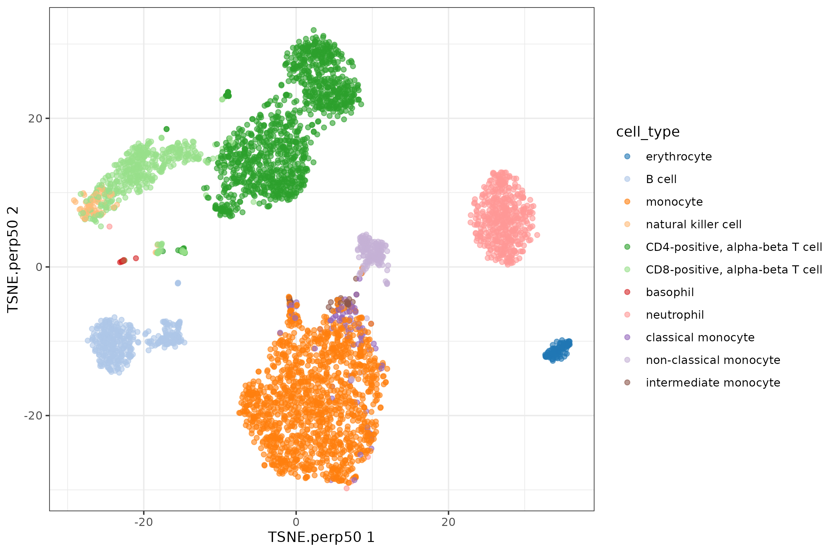
Perplexity 50 is the value that runTSNE would select for a dataset this big.

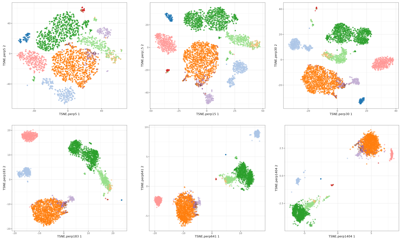
Now let's explore the rest of values, I selected a few

t-SNE perplexity,firs row shows values 5, 15 and 30. Second row 183, 641 and 1404

Now we focus on the theta parameter. This parameter is used to speed up the algorithm, but it can also affect the results. The default value is 0.5 so we will test values from 0 to 1. You see I did not included o.5 because I was used in the perplexity test. Here we will use perplexity 50.

 1for( t in  c(0, 0.25, 0.75, 1 ) ){
 2  pbmc.sce <- runTSNE( pbmc.sce,  
 3                           BPPARAM=BiocParallel::MulticoreParam(8), 
 4                           perplexity = 50,
 5                           theta = 0.5,
 6                           name = paste0( 'TSNE.theta', t )
 7  )
 8  g <- plotReducedDim( pbmc.sce, colour_by = 'cell_type', dimred = paste0( 'TSNE.theta', t ) ) +
 9    theme_bw()
10  ggsave( plot = g, filename = paste0( 'TSNE.theta', t, '.png' ), height = 5.86, width = 8.89 )
11}

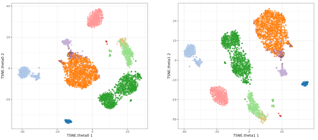
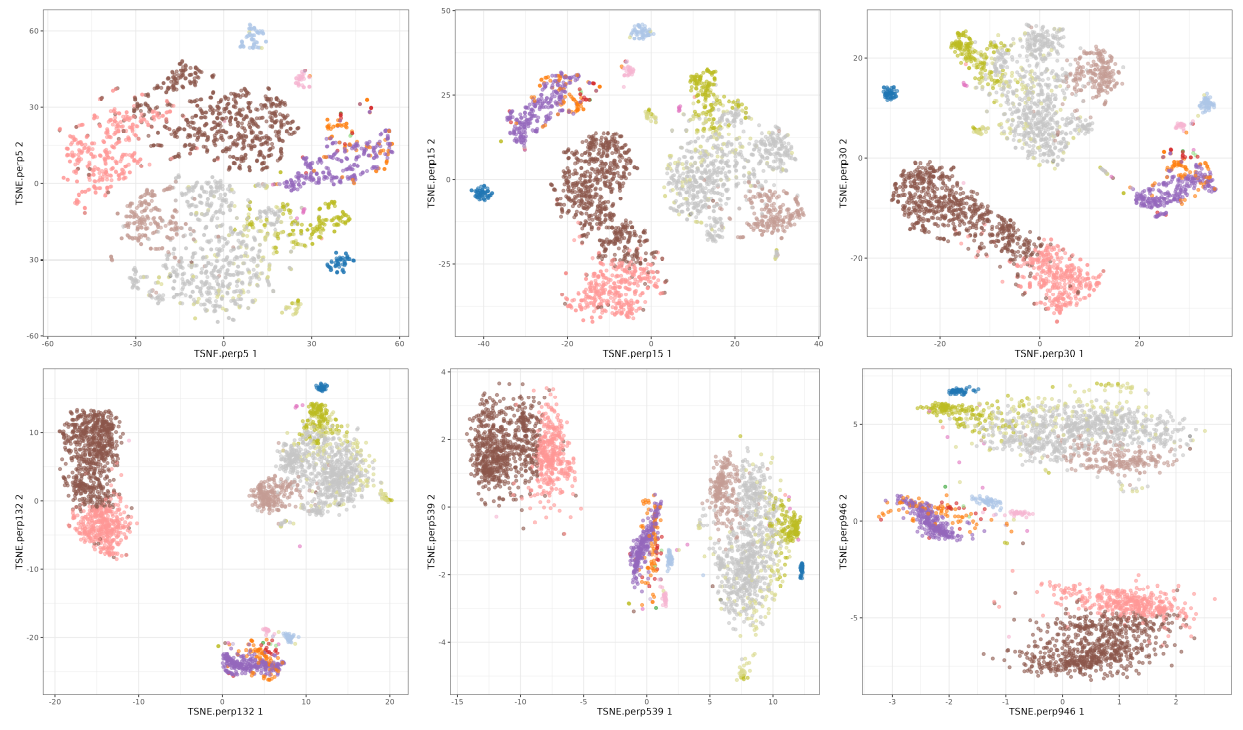
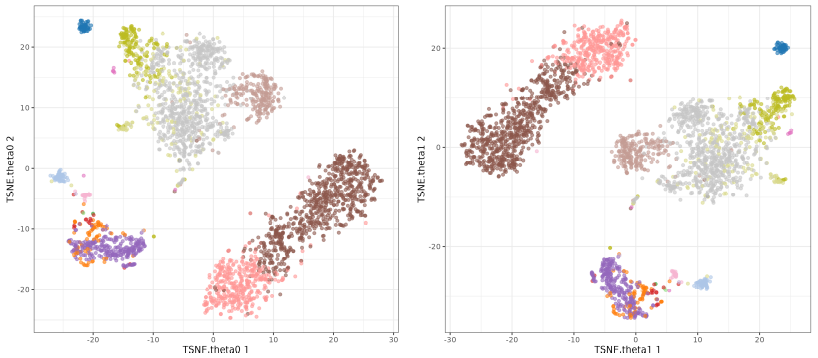
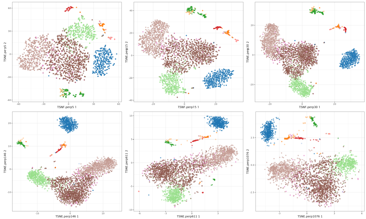
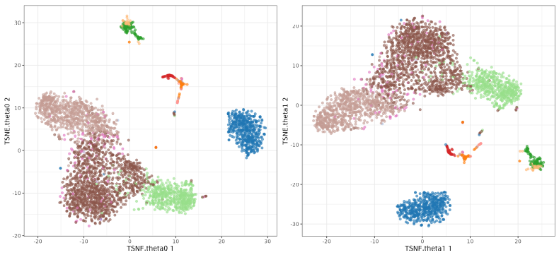
The perplexity tries to balance attention between local and global aspects of your data. Very low values seem to focus on local structure not showing main clusters of points, while very high values seem to miss relevant information showing 'over-condensed' clusters of cells. The theta parameter does not seem to affect too much to the main structure of the result.

UMAP

The runUMAP function calls the umap function from the uwot package, an R translation of the Python implementation of the original UMAP method.

UMAP algorithm has many parameters that can be tuned. I decided to focus on the number of neighbors (n_neighbors) and the minimum distance between embedded points (min_dist) sinde they have the greatest effect on the main of the output. More details here:

— n_neighbors: This parameter controls how UMAP balances local versus global structure in the data. It does this by constraining the size of the local neighborhood UMAP will look at when attempting to learn the manifold structure of the data. This means that low values of n_neighbors will force UMAP to concentrate on very local structure (potentially to the detriment of the big picture), while large values will push UMAP to look at larger neighborhoods of each point when estimating the manifold structure of the data, losing fine detail structure for the sake of getting the broader of the data. Default values is 15.
— min_dist: The min_dist parameter controls how tightly UMAP is allowed to pack points together. It, quite literally, provides the minimum distance apart that points are allowed to be in the low dimensional representation. This means that low values of min_dist will result in clumpier embeddings. This can be useful if you are interested in clustering, or in finer topological structure. Larger values of min_dist will prevent UMAP from packing points together and will focus on the preservation of the broad topological structure instead. Default values is 0.01,

 1for( k in c(5, 15, 30, 50, 100) ){
 2  for( d in c(0, 0.01, 0.05, 0.1, 0.5, 1)){
 3    pbmc.sce <- runUMAP( pbmc.sce, dimred = 'PCA', 
 4                             BPPARAM=BiocParallel::MulticoreParam(8), 
 5                             n_neighbors = k,
 6                             min_dist = d,
 7                             name = paste0( 'UMAP.neigh', k, '.dist', d )
 8                           )
 9    g <- plotReducedDim( pbmc.sce, colour_by = 'cell_type', dimred = paste0( 'UMAP.neigh', k, '.dist', d ) ) +
10      theme_bw()
11    ggsave( plot = g, filename = paste0( 'UMAP.neigh', k, '.dist', d, '.png' ), height = 5.86, width = 8.89 )
12  }
13}

Just by running the command we can already tell UMAP is way lighter on memory and faster than t-SNE.

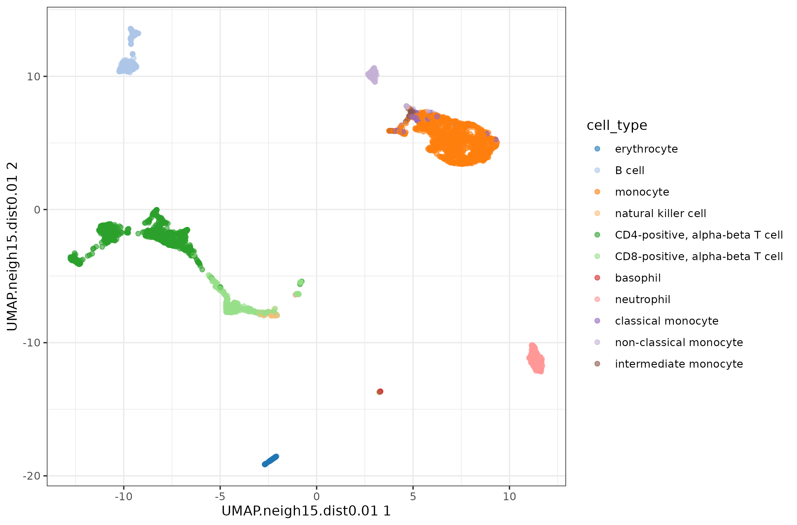
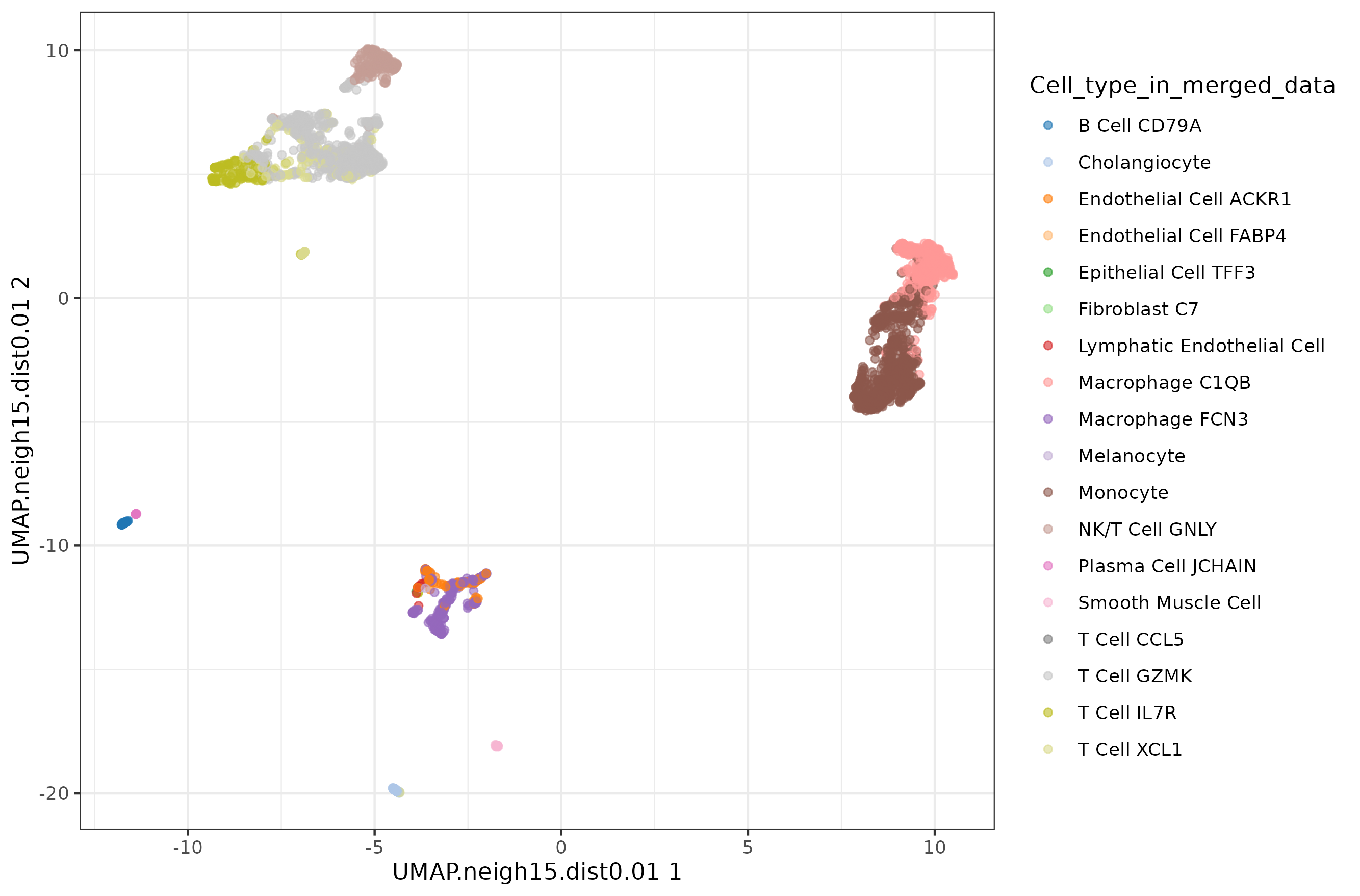
Let's check the default UMAP plot.

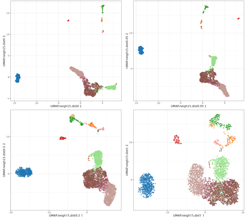
We first focus on the neighbors parameter.

UMAP neighbors,firs row shows values 5, 30. Second row 50 and 100

Now let's focus on min_dist parameter.

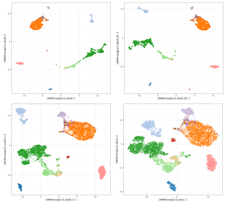
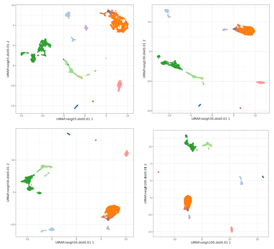
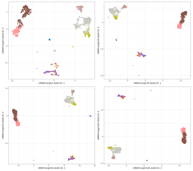
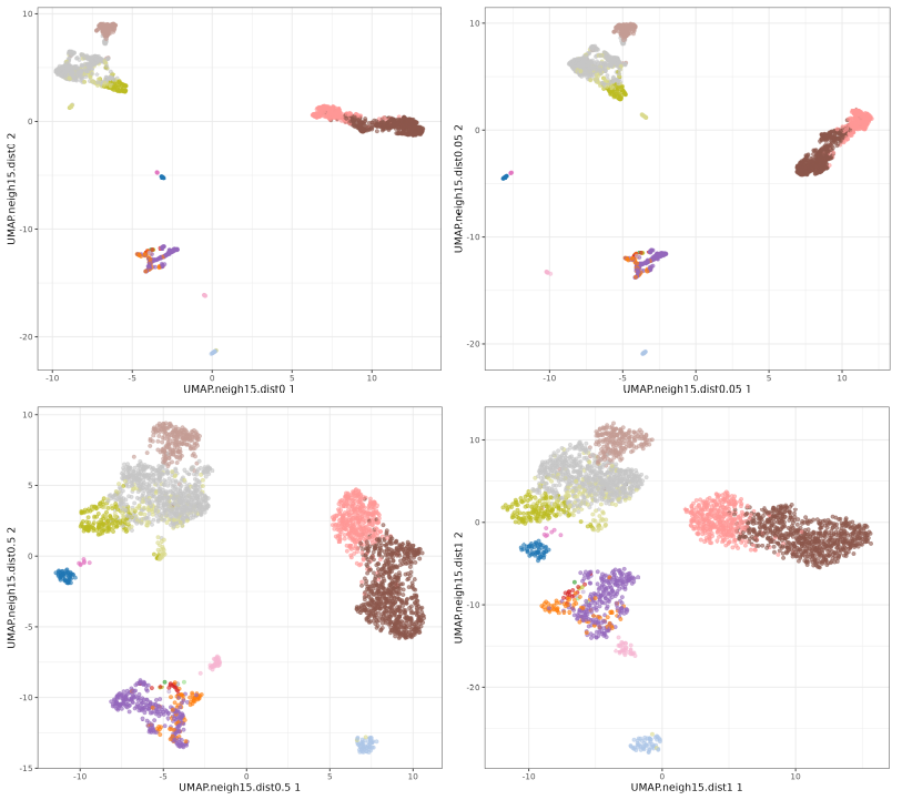
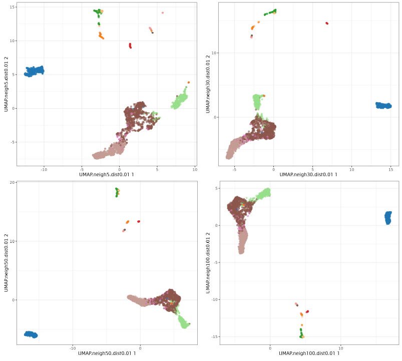
UMAP min_dist,firs row shows values 0, 0.05. Second row 0.5 and 1

The n_neighbors parameters does not seem to have much effect, just higher values 'compressing' a little bit more the clusters. The min_dist parameter has a more pronounced effect, with lower values showing more 'clumpy' clusters and higher values showing more 'spread' clusters.

Other datasets

I will use 2 datasets from the Human Cell Atlas, retrieved using the scRNAseq package.

1library(scRNAseq)

I defined function to perform the whole analysis, I will not show it here and leave that for you (you can see my function at the end of the post.)

Liver

1sce.liver <- fetchDataset("he-organs-2020","2023-12-21","liver")
2max_perp.liver <- (ncol(sce.liver) - 1) / 3
3sce.liver <- tSNE_UMAP( sce.liver, 'Cell_type_in_merged_data', max_perp.liver, 'liver' )

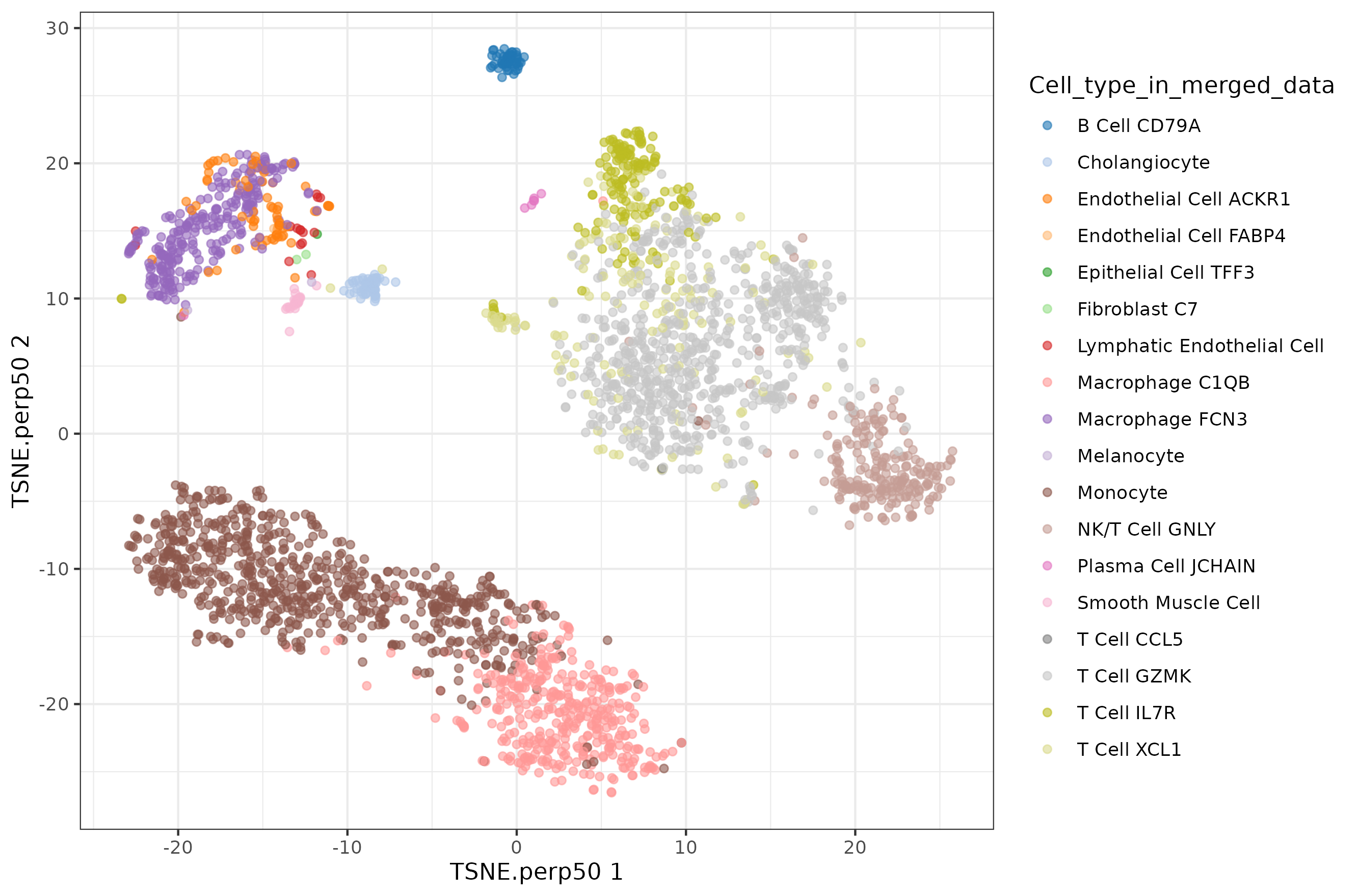
Default t-SNE

t-SNE perplexity

t-SNE theta

Default UMAP plot.

UMAP neighbors

UMAP min_dist parameter.

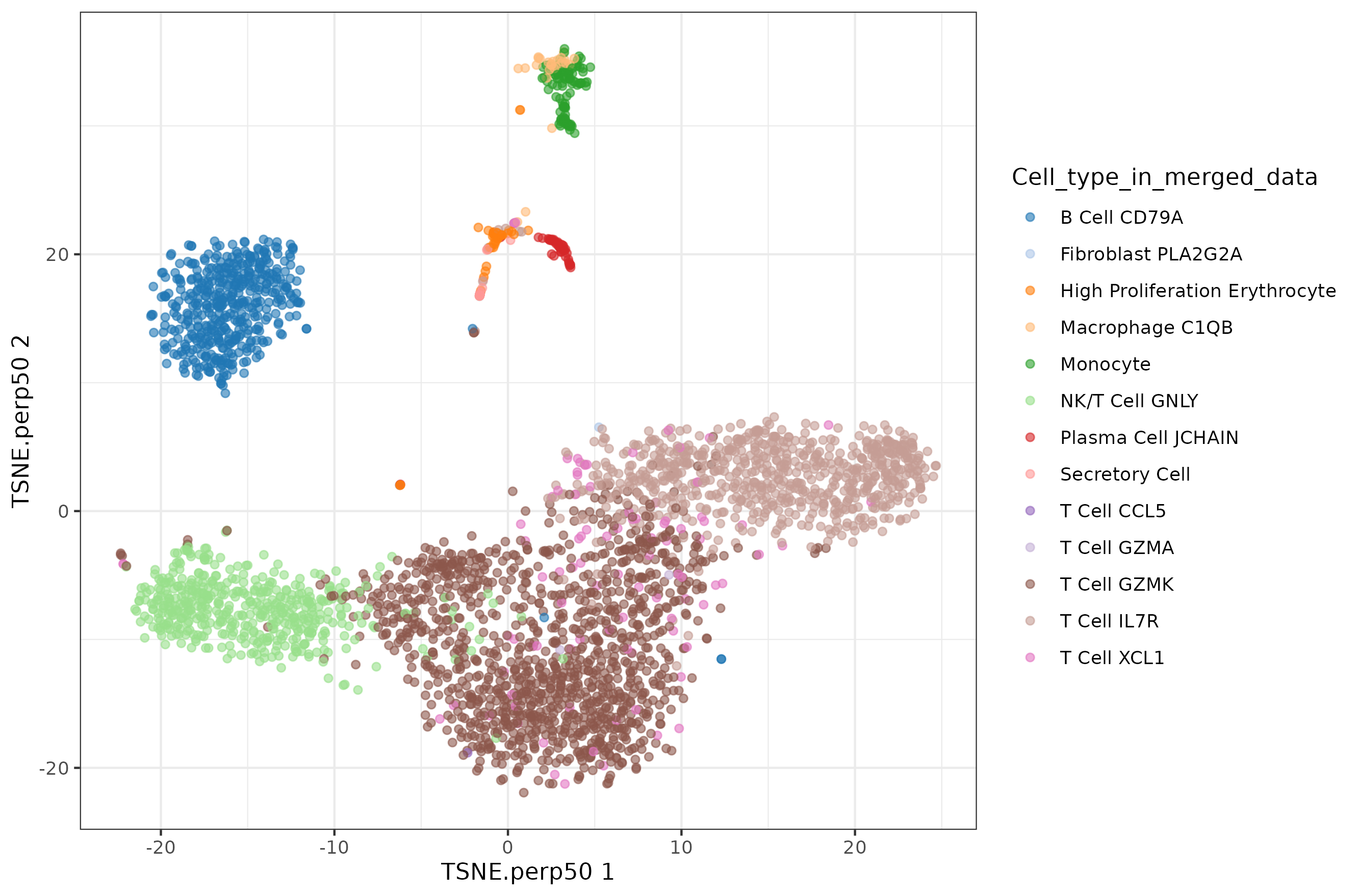
Bone Marrow

1sce.marrow <- fetchDataset("he-organs-2020","2023-12-21","marrow")
2max_perp.marrow <- (ncol(sce.marrow) - 1) / 3
3sce.marrow <- tSNE_UMAP( sce.marrow, 'Cell_type_in_merged_data', max_perp.marrow, 'marrow' )

Default t-SNE

Perplexity

t-SNE theta

UMAP neighbors

UMAP min_dist parameter.

Conclusions

Main cell type relationship does not change between t-SNE and UMAP suggesting both methods work reasonably well
The main parameter affecting t-SNE is perplexity
The main parameter affecting UMAP is min_dist
When using default values, the UMAP plot show more compact visual clusters with more empty blank background

Take away

Do not use t-SNE or UMAP coordinates for downstream analyses, use PCA coordinates instead
Do not over-interpret the results of t-SNE and UMAP and use them as a tool to visualize your data
Increasing min_dist in UMAP will make the result highly similar to the t-SNE result so in practical terms they are mostly equivalent
I tend to go with default parameters for both, t-SNE and UMAP, and then check if the cell grouping and relationship make sense. Then select the most visiually appealing plot.

Bonus I: UMAP perplexity

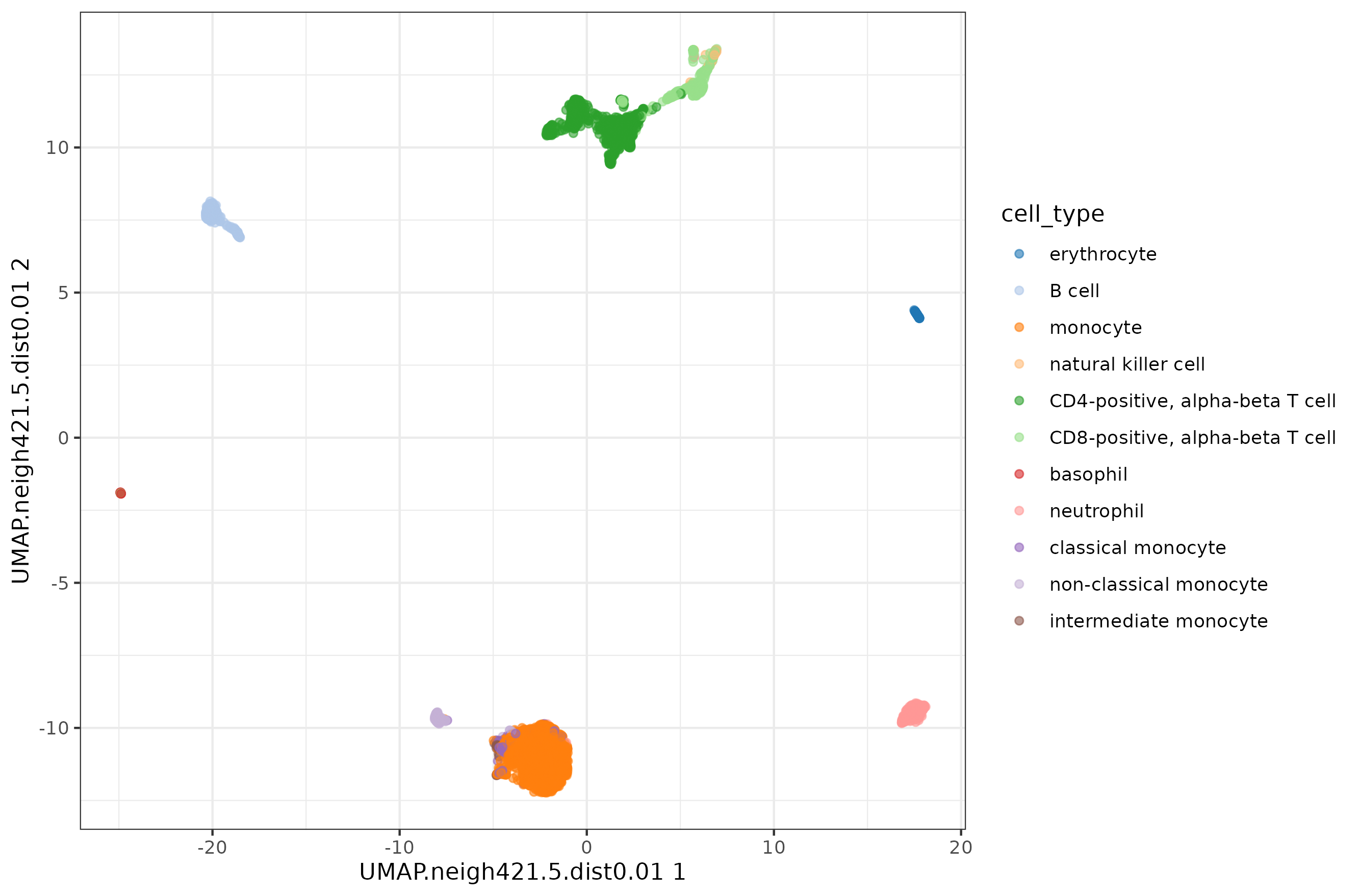
While finishing the writing of the post, I realized that the n_neighbors parameter options I chose might be too low for datasets with many cells. I decided to test a few more values for the blood dataset.

 1d <- 0.01
 2k <- ncol(pbmc.sce) / 10
 3
 4pbmc.sce <- runUMAP( pbmc.sce, dimred = 'PCA', 
 5                     BPPARAM=BiocParallel::MulticoreParam(8), 
 6                     n_neighbors = round(k,0),
 7                     min_dist = d,
 8                     name = paste0( 'UMAP.neigh', k, '.dist', d )
 9)
10
11plotReducedDim( pbmc.sce, colour_by = 'cell_type', dimred = paste0( 'UMAP.neigh', k, '.dist', d ) ) +
12  theme_bw()

 1d <- 0.01
 2k <- ncol(pbmc.sce) / 4
 3
 4pbmc.sce <- runUMAP( pbmc.sce, dimred = 'PCA', 
 5                     BPPARAM=BiocParallel::MulticoreParam(8), 
 6                     n_neighbors = round(k,0),
 7                     min_dist = d,
 8                     name = paste0( 'UMAP.neigh', k, '.dist', d )
 9)
10
11plotReducedDim( pbmc.sce, colour_by = 'cell_type', dimred = paste0( 'UMAP.neigh', k, '.dist', d ) ) +
12  theme_bw()

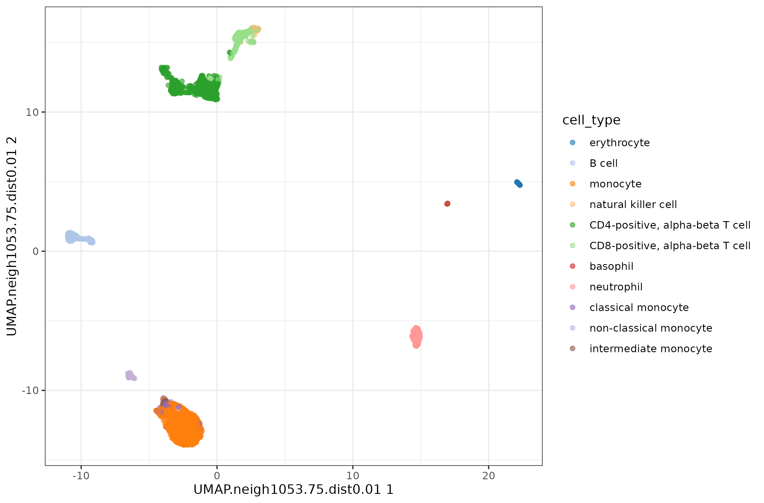
The conclusion remains the same, with very little difference in how compact the clusters look like.

Bonus II: Code solution

Here the code I used for the two Human Cell Atlas data sets.

 1tSNE_UMAP <- function( sce, celltype, max_perp, dataset.name ){
 2  # normalize
 3  sce.clusters <- quickCluster(sce, BPPARAM=BiocParallel::MulticoreParam(8))
 4  sce <- computeSumFactors( sce, 
 5                            cluster=sce.clusters, 
 6                            min.mean=0.1, 
 7                            BPPARAM=BiocParallel::MulticoreParam(8)
 8                          )
 9  sce <- logNormCounts( sce, BPPARAM=BiocParallel::MulticoreParam(8) )
10  dec.sce <- modelGeneVar( sce, BPPARAM=BiocParallel::MulticoreParam(8) )
11  top.HVGs <- getTopHVGs( dec.sce, n=2000 )
12  # PCA
13  sce <- runPCA( sce, 
14                 subset_row=top.HVGs, 
15                 BPPARAM=BiocParallel::MulticoreParam(8)
16               )
17  g <- plotPCA( sce, colour_by = celltype ) +
18    theme_bw()
19  ggsave( plot = g, filename = paste0( 'PCA.', dataset.name, '.png' ), height = 5.86, width = 8.89 )
20  # t-SNE
21  for( p in c(5, 10, 15, 50, seq( from = 30, to = max_perp, length.out = 10 ) ) ) {
22    p <- round(p, 0)
23    sce <- runTSNE( sce,  
24                         BPPARAM=BiocParallel::MulticoreParam(8), 
25                         perplexity = p,
26                         name = paste0( 'TSNE.perp', p )
27    )
28    g <- plotReducedDim( sce, colour_by = celltype, dimred = paste0( 'TSNE.perp', p ) ) +
29      theme_bw()
30    ggsave( plot = g, filename = paste0( 'TSNE.perp', p, '.', dataset.name, '.png' ), height = 5.86, width = 8.89 )
31  }
32  for( t in  c(0, 0.25, 0.75, 1 ) ){
33    sce <- runTSNE( sce,  
34                         BPPARAM=BiocParallel::MulticoreParam(8), 
35                         perplexity = 50,
36                         theta = 0.5,
37                         name = paste0( 'TSNE.theta', t )
38    )
39    g <- plotReducedDim( sce, colour_by = celltype, dimred = paste0( 'TSNE.theta', t ) ) +
40      theme_bw()
41    ggsave( plot = g, filename = paste0( 'TSNE.theta', t, '.', dataset.name, '.png' ), height = 5.86, width = 8.89 )
42  }
43  # UMAP
44  for( k in c(5, 15, 30, 50, 100) ){
45    for( d in c(0, 0.01, 0.05, 0.1, 0.5, 1)){
46      sce <- runUMAP( sce, dimred = 'PCA', 
47                           BPPARAM=BiocParallel::MulticoreParam(8), 
48                           n_neighbors = k,
49                           min_dist = d,
50                           name = paste0( 'UMAP.neigh', k, '.dist', d )
51      )
52      g <- plotReducedDim( sce, colour_by = celltype, dimred = paste0( 'UMAP.neigh', k, '.dist', d ) ) +
53        theme_bw()
54      ggsave( plot = g, filename = paste0( 'UMAP.neigh', k, '.dist', d, '.', dataset.name, '.png' ), height = 5.86, width = 8.89 )
55    }
56  }
57  return(sce)
58}