Pairwise Controlled Manifold Approximation (PaCMAP) for Single Cell
While preparing my posts on t-SNE vs UMAP and Phate I found this paper, which introduced a new dimensional reduction method called PaCMAP (Pairwise Controlled Manifold Approximation) and compared it with tSNE, UMAP, and other methods I did not know.

According to the paper, PaCMAP is a new method preserves both local and global structure in high-dimensional data, making it particularly suitable for single-cell RNA-seq data visualization. It is designed to overcome some of the limitations of existing methods like t-SNE and UMAP, such as sensitivity to parameter settings and computational efficiency. After reading this, I decided to give it a try.
It is a python package so I installed in a dedicated virtual environment to avoid issues with other packages.
1mkvirtualenv pacmap
2pip install pacmap
I use reticulate R pacakge to manage the communication of R and the Python virtual environment. Run this chunk at the begining to avoid issues.
1reticulate::use_virtualenv("~/.virtualenvs/pacmap", required = TRUE)
2reticulate::py_config()
1## python:         /home/alfonso/.virtualenvs/pacmap/bin/python
2## libpython:      /usr/lib/python3.10/config-3.10-x86_64-linux-gnu/libpython3.10.so
3## pythonhome:     /home/alfonso/.virtualenvs/pacmap:/home/alfonso/.virtualenvs/pacmap
4## virtualenv:     /home/alfonso/.virtualenvs/pacmap/bin/activate_this.py
5## version:        3.10.12 (main, May 27 2025, 17:12:29) [GCC 11.4.0]
6## numpy:          /home/alfonso/.virtualenvs/pacmap/lib/python3.10/site-packages/numpy
7## numpy_version:  2.2.6
8##
9## NOTE: Python version was forced by use_python() function
I will use our good old friend, the dataset of blood cells from the cellxgene database that I used in many of my previous posts such as Scanpy, Seurat or SCE.
The following code reads and filters the dataset. See my previous posts for more details.
1library(Seurat)
2rds.file <- file.path( '582149d8-2a8f-44cf-9605-337b8ca8d518.rds' )
3seurat <- readRDS(rds.file)
 1library(dplyr)
 2library(tidyr)
 3library(tidylog)
 4keep.cells <- seurat[[]] %>%
 5  tibble::rownames_to_column( 'Cell' ) %>%
 6  filter( assay == "10x 3' v3", donor_id == 'TSP1' ) %>%
 7  group_by( cell_type ) %>%
 8  mutate( tot = n() ) %>%
 9  filter( tot >= 20 )
10
11pbmc <- subset(seurat, cells = keep.cells$Cell)
12dim(pbmc)
1## [1] 61759 4215
Since the PaCMAP algorithm is implemented in Python, I will use an R wrapper, part of the SeuratWrappers package so I will preprocess the object using the Seurat workflow. If you are not familiar with Seurat, I recommend you to read my previous post on Seurat first.
Before starting, we must convert the Seurat object to the Seurat v5.2.1 structure.
1pbmc <- UpdateSeuratObject(pbmc)
1## Validating object structure
1## Updating object slots
1## Ensuring keys are in the proper structure
1## Updating matrix keys for DimReduc 'pca'
1## Updating matrix keys for DimReduc 'scvi'
1## Updating matrix keys for DimReduc 'tissue_uncorrected_umap'
1## Updating matrix keys for DimReduc 'umap'
1## Updating matrix keys for DimReduc 'umap_scvi_full_donorassay'
1## Updating matrix keys for DimReduc 'umap_tissue_scvi_donorassay'
1## Updating matrix keys for DimReduc 'uncorrected_umap'
1## Ensuring keys are in the proper structure
1## Ensuring feature names don't have underscores or pipes
1## Updating slots in RNA
1## Updating slots in pca
1## Updating slots in scvi
1## Updating slots in tissue_uncorrected_umap
1## Setting tissue_uncorrected_umap DimReduc to global
1## Updating slots in umap
1## Setting umap DimReduc to global
1## Updating slots in umap_scvi_full_donorassay
1## Setting umap_scvi_full_donorassay DimReduc to global
1## Updating slots in umap_tissue_scvi_donorassay
1## Setting umap_tissue_scvi_donorassay DimReduc to global
1## Updating slots in uncorrected_umap
1## Setting uncorrected_umap DimReduc to global
1## Validating object structure for Assay 'RNA'
1## Validating object structure for DimReduc 'pca'
1## Validating object structure for DimReduc 'scvi'
1## Validating object structure for DimReduc 'tissue_uncorrected_umap'
1## Validating object structure for DimReduc 'umap'
1## Validating object structure for DimReduc 'umap_scvi_full_donorassay'
1## Validating object structure for DimReduc 'umap_tissue_scvi_donorassay'
1## Validating object structure for DimReduc 'uncorrected_umap'
1## Object representation is consistent with the most current Seurat version
1pbmc
1## An object of class Seurat
2## 61759 features across 4215 samples within 1 assay
3## Active assay: RNA (61759 features, 0 variable features)
4##  2 layers present: counts, data
5##  7 dimensional reductions calculated: pca, scvi, tissue_uncorrected_umap, umap, umap_scvi_full_donorassay, umap_tissue_scvi_donorassay, uncorrected_umap
QC evaluation
1mito.genes <- pbmc[['RNA']][[]] %>%
2  as.data.frame() %>%
3  filter( mt == T ) %>%
4  tibble::rownames_to_column( 'gene' ) %>%
5  pull('gene')
1## filter: removed 61,722 rows (>99%), 37 rows remaining
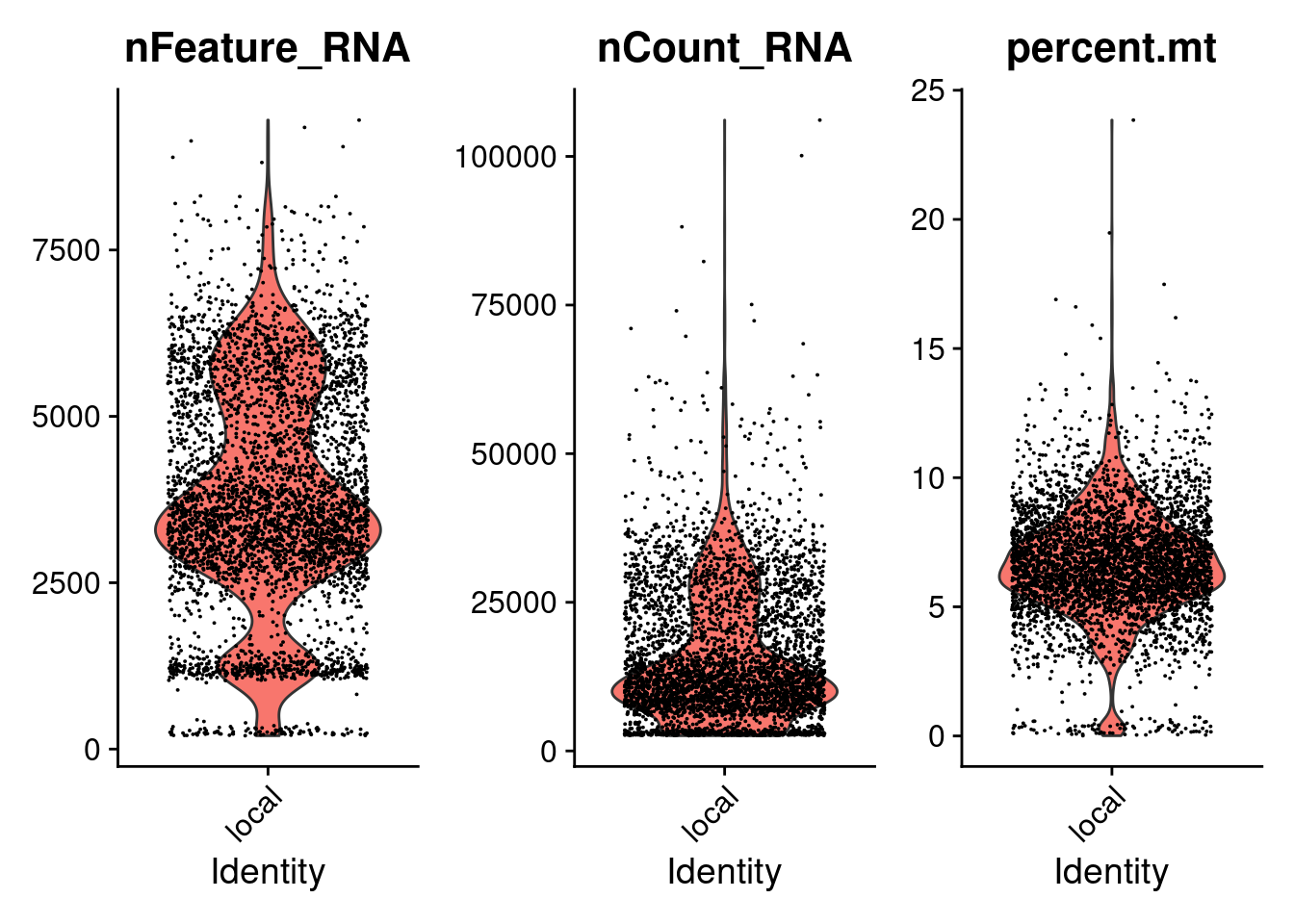
1pbmc[["percent.mt"]] <- PercentageFeatureSet(pbmc, features = mito.genes)
2# Visualize QC metrics as a violin plot
3VlnPlot(pbmc, features = c("nFeature_RNA", "nCount_RNA", "percent.mt"), ncol = 3)
1## Warning: The `slot` argument of `FetchData()` is deprecated as of SeuratObject 5.0.0.
2## ℹ Please use the `layer` argument instead.
3## ℹ The deprecated feature was likely used in the Seurat package.
4##   Please report the issue at <https://github.com/satijalab/seurat/issues>.
5## This warning is displayed once every 8 hours.
6## Call `lifecycle::last_lifecycle_warnings()` to see where this warning was
7## generated.
1## Warning: `PackageCheck()` was deprecated in SeuratObject 5.0.0.
2## ℹ Please use `rlang::check_installed()` instead.
3## ℹ The deprecated feature was likely used in the Seurat package.
4##   Please report the issue at <https://github.com/satijalab/seurat/issues>.
5## This warning is displayed once every 8 hours.
6## Call `lifecycle::last_lifecycle_warnings()` to see where this warning was
7## generated.
1FeatureScatter(pbmc, feature1 = "nCount_RNA", feature2 = "nFeature_RNA", group.by = 'cell_type' )
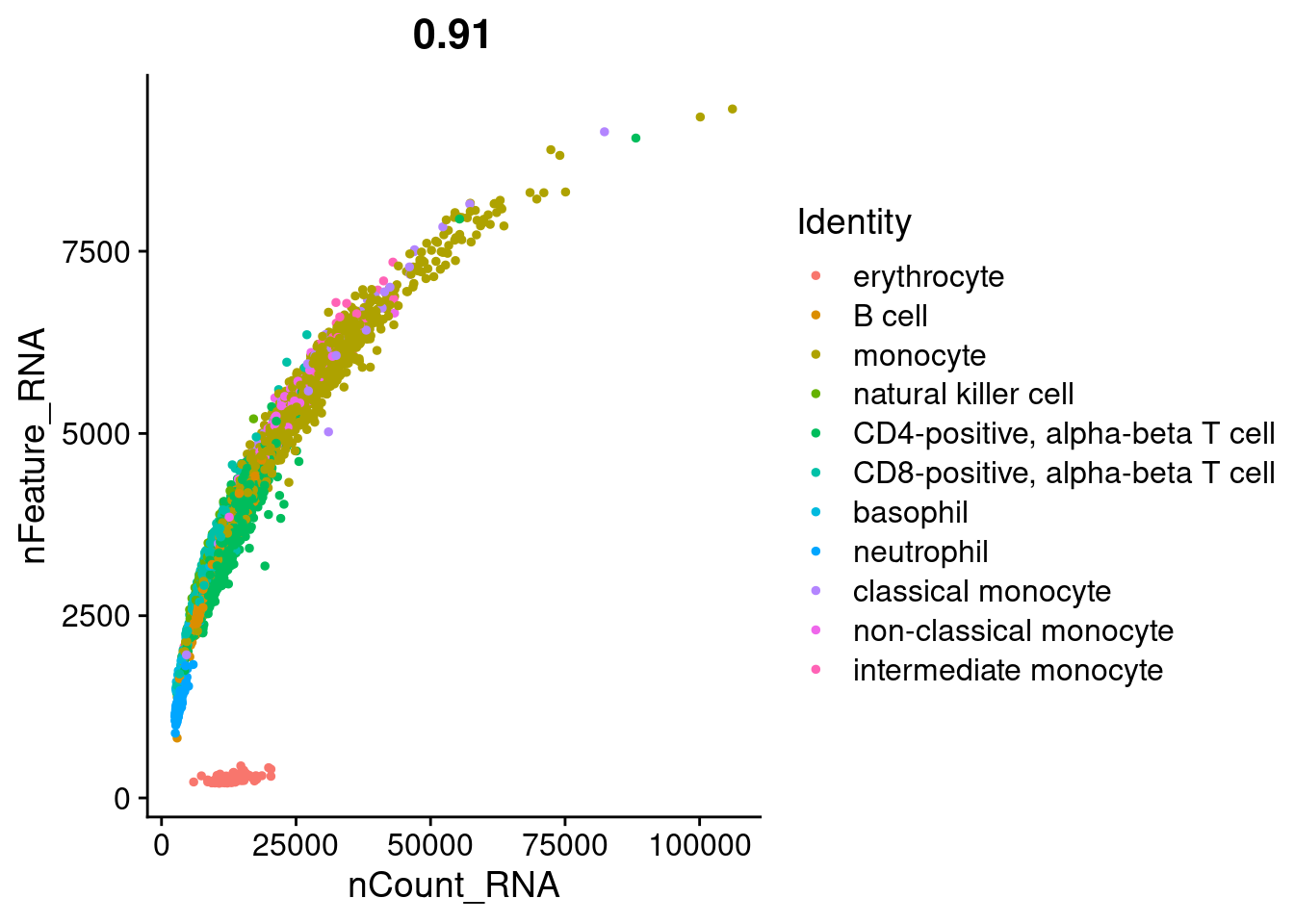
As expected, red blood cells have low number of features and counts.
I would like to evaluate the percent mito in the previous plot. By default, FeatureScatter() does not support a color.by argument for numerial values, we can work around this easily by extracting the data and using ggplot2.
1library(ggplot2)
2plot_df <- FetchData(pbmc, vars = c("nCount_RNA", "nFeature_RNA", "percent.mt"))
3ggplot(plot_df, aes(x = nCount_RNA, y = nFeature_RNA, color = percent.mt)) +
4  geom_point(size = 1) +
5  scale_color_viridis_c() +
6  theme_bw() +
7  labs(color = "% mito", x = "nCount_RNA", y = "nFeature_RNA")

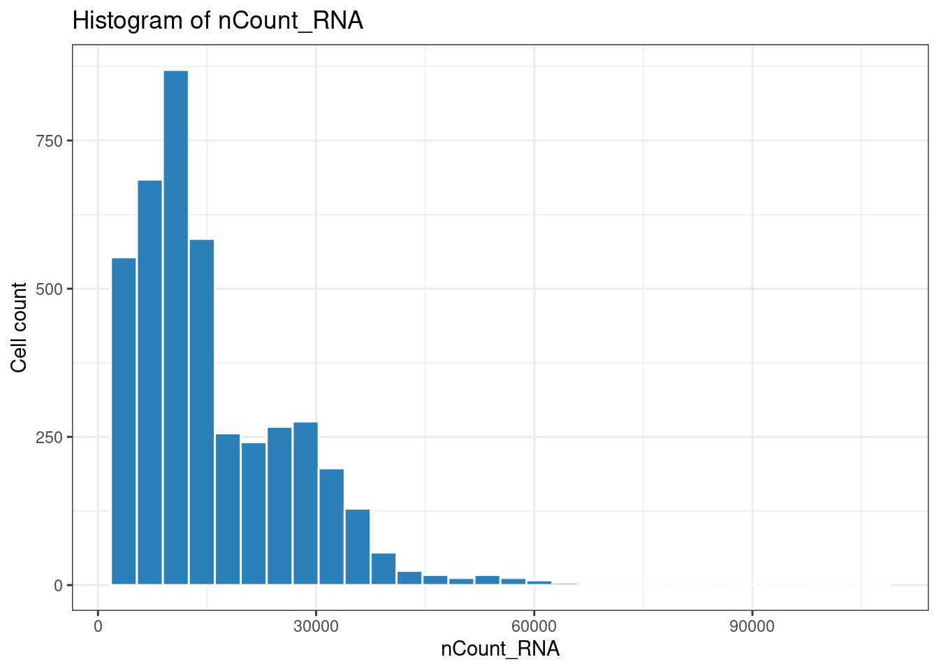
1ggplot(plot_df, aes(x = nCount_RNA)) +
2  geom_histogram(fill = "#2c7fb8", color = "white") +
3  theme_bw() +
4  labs(title = "Histogram of nCount_RNA", x = "nCount_RNA", y = "Cell count")
1## `stat_bin()` using `bins = 30`. Pick better value with `binwidth`.
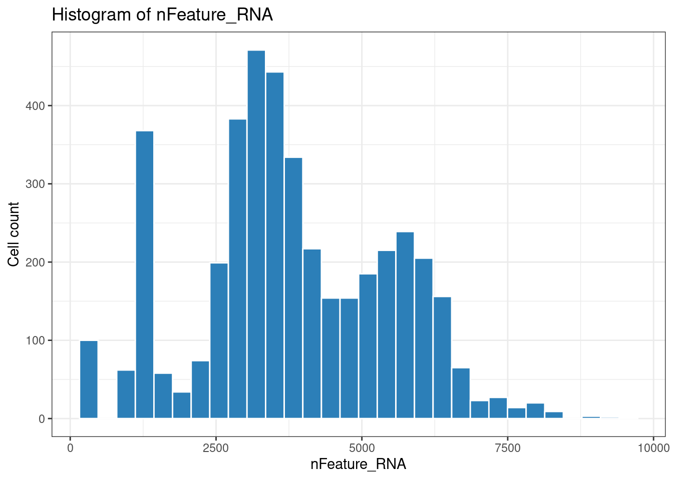
1ggplot(plot_df, aes(x = nFeature_RNA)) +
2  geom_histogram(fill = "#2c7fb8", color = "white") +
3  theme_bw() +
4  labs(title = "Histogram of nFeature_RNA", x = "nFeature_RNA", y = "Cell count")
1## `stat_bin()` using `bins = 30`. Pick better value with `binwidth`.
1ggplot(plot_df, aes(x = percent.mt)) +
2  geom_histogram(fill = "#2c7fb8", color = "white") +
3  theme_bw() +
4  labs(title = "Histogram of percent.mt", x = "percent.mt", y = "Cell count")
1## `stat_bin()` using `bins = 30`. Pick better value with `binwidth`.

Usually we would filter based on genes, umis and mt percentage, depending on the experimental settings. Since we are using cellxgene data, and to keep the red blood cells, I will use only a soft mitochondrial threshold.
1pbmc <- subset(pbmc, subset = percent.mt < 15)
2dim(pbmc)
1## [1] 61759 4207
Normalize data
1pbmc <- NormalizeData(pbmc)
1## Warning: The `slot` argument of `SetAssayData()` is deprecated as of SeuratObject 5.0.0.
2## ℹ Please use the `layer` argument instead.
3## ℹ The deprecated feature was likely used in the Seurat package.
4##   Please report the issue at <https://github.com/satijalab/seurat/issues>.
5## This warning is displayed once every 8 hours.
6## Call `lifecycle::last_lifecycle_warnings()` to see where this warning was
7## generated.
1## Warning: The `slot` argument of `GetAssayData()` is deprecated as of SeuratObject 5.0.0.
2## ℹ Please use the `layer` argument instead.
3## ℹ The deprecated feature was likely used in the Seurat package.
4##   Please report the issue at <https://github.com/satijalab/seurat/issues>.
5## This warning is displayed once every 8 hours.
6## Call `lifecycle::last_lifecycle_warnings()` to see where this warning was
7## generated.
Find high variable genes for PCA
1pbmc <- FindVariableFeatures(pbmc, selection.method = "vst", nfeatures = 2000)
Scale data
1pbmc <- ScaleData(pbmc, features = rownames(pbmc) )
1## Centering and scaling data matrix
Run PCA
1pbmc <- RunPCA(pbmc, features = VariableFeatures(object = pbmc))
 1## PC_ 1
 2## Positive:  ENSG00000085265, ENSG00000163131, ENSG00000120594, ENSG00000197249, ENSG00000087086, ENSG00000011600, ENSG00000090382, ENSG00000148655, ENSG00000101439, ENSG00000172322
 3## 	   ENSG00000030582, ENSG00000204472, ENSG00000158869, ENSG00000025708, ENSG00000170458, ENSG00000197746, ENSG00000163220, ENSG00000038427, ENSG00000172243, ENSG00000121552
 4## 	   ENSG00000170345, ENSG00000123384, ENSG00000127951, ENSG00000257764, ENSG00000165168, ENSG00000090376, ENSG00000163563, ENSG00000104093, ENSG00000197629, ENSG00000113269
 5## Negative:  ENSG00000127152, ENSG00000198821, ENSG00000008517, ENSG00000165929, ENSG00000113263, ENSG00000211772, ENSG00000277734, ENSG00000227507, ENSG00000171791, ENSG00000153283
 6## 	   ENSG00000069667, ENSG00000168685, ENSG00000161405, ENSG00000172673, ENSG00000152495, ENSG00000151150, ENSG00000109452, ENSG00000205045, ENSG00000081059, ENSG00000237943
 7## 	   ENSG00000289740, ENSG00000138378, ENSG00000138795, ENSG00000112182, ENSG00000151623, ENSG00000126353, ENSG00000173762, ENSG00000135426, ENSG00000163519, ENSG00000099204
 8## PC_ 2
 9## Positive:  ENSG00000153064, ENSG00000105369, ENSG00000156738, ENSG00000247982, ENSG00000144218, ENSG00000196092, ENSG00000167483, ENSG00000144645, ENSG00000211899, ENSG00000012124
10## 	   ENSG00000007312, ENSG00000164330, ENSG00000095585, ENSG00000136573, ENSG00000204287, ENSG00000163534, ENSG00000019582, ENSG00000196735, ENSG00000211898, ENSG00000119866
11## 	   ENSG00000179344, ENSG00000082293, ENSG00000112232, ENSG00000042980, ENSG00000176533, ENSG00000116191, ENSG00000231389, ENSG00000289963, ENSG00000081189, ENSG00000116194
12## Negative:  ENSG00000008517, ENSG00000198821, ENSG00000077984, ENSG00000127152, ENSG00000113263, ENSG00000165929, ENSG00000205045, ENSG00000277734, ENSG00000153283, ENSG00000172673
13## 	   ENSG00000138378, ENSG00000122862, ENSG00000168685, ENSG00000237943, ENSG00000109452, ENSG00000152495, ENSG00000069667, ENSG00000152270, ENSG00000173762, ENSG00000059804
14## 	   ENSG00000164483, ENSG00000138795, ENSG00000211751, ENSG00000163421, ENSG00000145819, ENSG00000074966, ENSG00000172543, ENSG00000163519, ENSG00000135636, ENSG00000123146
15## PC_ 3
16## Positive:  ENSG00000197747, ENSG00000084207, ENSG00000124942, ENSG00000182718, ENSG00000213145, ENSG00000197471, ENSG00000108798, ENSG00000168329, ENSG00000125148, ENSG00000156299
17## 	   ENSG00000182578, ENSG00000137486, ENSG00000175198, ENSG00000281103, ENSG00000198821, ENSG00000100097, ENSG00000119655, ENSG00000106066, ENSG00000008517, ENSG00000196230
18## 	   ENSG00000115738, ENSG00000166927, ENSG00000182621, ENSG00000104972, ENSG00000198879, ENSG00000163590, ENSG00000105374, ENSG00000114013, ENSG00000155366, ENSG00000170315
19## Negative:  ENSG00000162747, ENSG00000162551, ENSG00000163421, ENSG00000257335, ENSG00000140932, ENSG00000157551, ENSG00000196549, ENSG00000115590, ENSG00000151726, ENSG00000163993
20## 	   ENSG00000135636, ENSG00000100985, ENSG00000248323, ENSG00000286076, ENSG00000203710, ENSG00000204936, ENSG00000059804, ENSG00000115594, ENSG00000143797, ENSG00000183762
21## 	   ENSG00000105835, ENSG00000234426, ENSG00000127954, ENSG00000291237, ENSG00000183019, ENSG00000163221, ENSG00000146592, ENSG00000009694, ENSG00000111052, ENSG00000159339
22## PC_ 4
23## Positive:  ENSG00000172005, ENSG00000138795, ENSG00000186854, ENSG00000126353, ENSG00000152495, ENSG00000109452, ENSG00000163519, ENSG00000081059, ENSG00000249806, ENSG00000182463
24## 	   ENSG00000141576, ENSG00000290067, ENSG00000227507, ENSG00000168685, ENSG00000249859, ENSG00000091409, ENSG00000165591, ENSG00000107104, ENSG00000189283, ENSG00000165272
25## 	   ENSG00000246223, ENSG00000184613, ENSG00000111863, ENSG00000197635, ENSG00000151150, ENSG00000170074, ENSG00000135426, ENSG00000271774, ENSG00000232021, ENSG00000237943
26## Negative:  ENSG00000105374, ENSG00000115523, ENSG00000134539, ENSG00000100453, ENSG00000180644, ENSG00000145649, ENSG00000137441, ENSG00000100450, ENSG00000275302, ENSG00000116667
27## 	   ENSG00000271503, ENSG00000069702, ENSG00000107719, ENSG00000150045, ENSG00000171476, ENSG00000181036, ENSG00000159618, ENSG00000205336, ENSG00000170962, ENSG00000156475
28## 	   ENSG00000077984, ENSG00000159674, ENSG00000168229, ENSG00000251301, ENSG00000185697, ENSG00000150687, ENSG00000104490, ENSG00000235162, ENSG00000169583, ENSG00000172543
29## PC_ 5
30## Positive:  ENSG00000129757, ENSG00000287682, ENSG00000188290, ENSG00000107954, ENSG00000157827, ENSG00000203747, ENSG00000180229, ENSG00000142089, ENSG00000233392, ENSG00000148737
31## 	   ENSG00000214407, ENSG00000183779, ENSG00000166165, ENSG00000166068, ENSG00000135047, ENSG00000259225, ENSG00000224397, ENSG00000258732, ENSG00000155366, ENSG00000123358
32## 	   ENSG00000229140, ENSG00000166927, ENSG00000182578, ENSG00000170873, ENSG00000142512, ENSG00000120949, ENSG00000074416, ENSG00000106341, ENSG00000107736, ENSG00000226321
33## Negative:  ENSG00000120885, ENSG00000008394, ENSG00000138061, ENSG00000135218, ENSG00000038427, ENSG00000121807, ENSG00000169385, ENSG00000257764, ENSG00000164125, ENSG00000182621
34## 	   ENSG00000136830, ENSG00000135046, ENSG00000161944, ENSG00000164124, ENSG00000090382, ENSG00000120738, ENSG00000121316, ENSG00000105967, ENSG00000010327, ENSG00000226822
35## 	   ENSG00000186815, ENSG00000157168, ENSG00000110077, ENSG00000104918, ENSG00000257017, ENSG00000125740, ENSG00000177575, ENSG00000128487, ENSG00000170458, ENSG00000178695
1DimPlot(pbmc, reduction = "pca", group.by = 'cell_type')

Run UMAP, for this quick test I will use all PCs
1pbmc <- RunUMAP(pbmc, dims = 1:50)
1## Warning: The default method for RunUMAP has changed from calling Python UMAP via reticulate to the R-native UWOT using the cosine metric
2## To use Python UMAP via reticulate, set umap.method to 'umap-learn' and metric to 'correlation'
3## This message will be shown once per session
1## 17:13:37 UMAP embedding parameters a = 0.9922 b = 1.112
1## 17:13:37 Read 4207 rows and found 50 numeric columns
1## 17:13:37 Using Annoy for neighbor search, n_neighbors = 30
1## 17:13:37 Building Annoy index with metric = cosine, n_trees = 50
1## 0% 10 20 30 40 50 60 70 80 90 100%
1## [----|----|----|----|----|----|----|----|----|----|
1## **************************************************|
2## 17:13:37 Writing NN index file to temp file /tmp/RtmpRhKGc1/file14a1d62c832e8c
3## 17:13:37 Searching Annoy index using 1 thread, search_k = 3000
4## 17:13:38 Annoy recall = 100%
5## 17:13:38 Commencing smooth kNN distance calibration using 1 thread with target n_neighbors = 30
6## 17:13:38 Initializing from normalized Laplacian + noise (using RSpectra)
7## 17:13:39 Commencing optimization for 500 epochs, with 175432 positive edges
8## 17:13:39 Using rng type: pcg
9## 17:13:43 Optimization finished
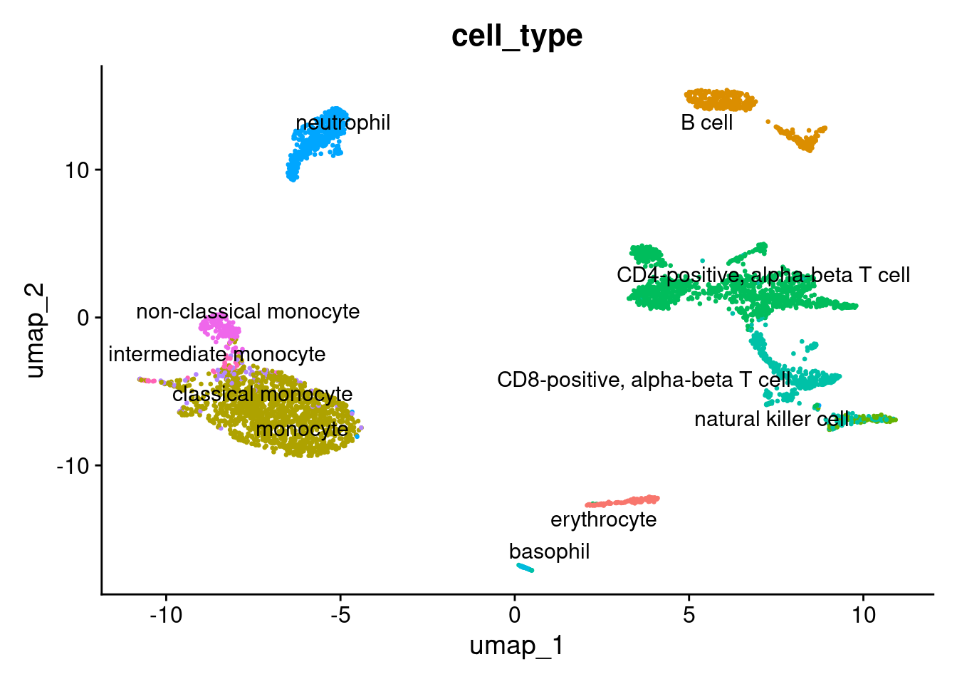
Plot UMAP
1DimPlot(pbmc, reduction = "umap", label = TRUE, repel = TRUE, group.by = 'cell_type' ) + NoLegend()
Run PaCMAP using the SeuratWrappers package.
1# remotes::install_github('satijalab/seurat-wrappers')
2library(SeuratWrappers)
3pbmc <- RunPaCMAP(object = pbmc, features = Seurat::VariableFeatures(pbmc))
 1## Applied PCA, the dimensionality becomes 100
 2## PaCMAP(n_neighbors=10, n_MN=5, n_FP=20, distance=euclidean, lr=1.0, n_iters=(100, 100, 250), apply_pca=True, opt_method='adam', verbose=True, intermediate=False, seed=11)
 3## Finding pairs
 4## Found nearest neighbor
 5## Calculated sigma
 6## Found scaled dist
 7## Pairs sampled successfully.
 8## ((42070, 2), (21035, 2), (84140, 2))
 9## Initial Loss: 51819.17578125
10## Iteration:   10, Loss: 39982.265625
11## Iteration:   20, Loss: 31825.072266
12## Iteration:   30, Loss: 29064.273438
13## Iteration:   40, Loss: 27609.316406
14## Iteration:   50, Loss: 26209.269531
15## Iteration:   60, Loss: 24828.828125
16## Iteration:   70, Loss: 23298.683594
17## Iteration:   80, Loss: 21438.656250
18## Iteration:   90, Loss: 19014.822266
19## Iteration:  100, Loss: 15215.458984
20## Iteration:  110, Loss: 18434.947266
21## Iteration:  120, Loss: 18176.066406
22## Iteration:  130, Loss: 18079.007812
23## Iteration:  140, Loss: 18039.667969
24## Iteration:  150, Loss: 18020.625000
25## Iteration:  160, Loss: 18009.695312
26## Iteration:  170, Loss: 18001.855469
27## Iteration:  180, Loss: 17995.763672
28## Iteration:  190, Loss: 17990.417969
29## Iteration:  200, Loss: 17984.171875
30## Iteration:  210, Loss: 8186.588379
31## Iteration:  220, Loss: 8046.067871
32## Iteration:  230, Loss: 7987.240234
33## Iteration:  240, Loss: 7946.288086
34## Iteration:  250, Loss: 7918.241211
35## Iteration:  260, Loss: 7897.881348
36## Iteration:  270, Loss: 7881.938477
37## Iteration:  280, Loss: 7868.776367
38## Iteration:  290, Loss: 7857.554199
39## Iteration:  300, Loss: 7847.858398
40## Iteration:  310, Loss: 7839.208008
41## Iteration:  320, Loss: 7831.520020
42## Iteration:  330, Loss: 7824.563477
43## Iteration:  340, Loss: 7818.220215
44## Iteration:  350, Loss: 7812.399414
45## Iteration:  360, Loss: 7806.992188
46## Iteration:  370, Loss: 7802.010742
47## Iteration:  380, Loss: 7797.365723
48## Iteration:  390, Loss: 7793.033691
49## Iteration:  400, Loss: 7788.949219
50## Iteration:  410, Loss: 7785.119141
51## Iteration:  420, Loss: 7781.532227
52## Iteration:  430, Loss: 7778.101562
53## Iteration:  440, Loss: 7774.856445
54## Iteration:  450, Loss: 7771.775879
55## Elapsed time: 0.86s
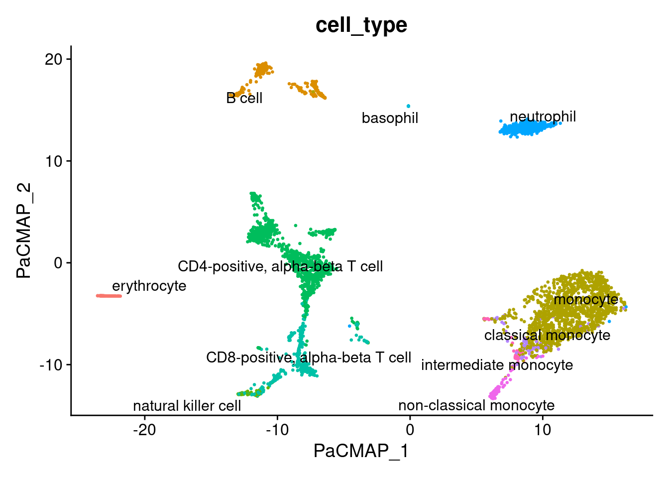
Plot PaCMAP
1DimPlot(pbmc, reduction="pacmap", label = TRUE, repel = TRUE, group.by = 'cell_type' ) + NoLegend()
Other datasets
I will use 2 datasets from the Human Cell Atlas, retrieved using the scRNAseq package.
1library(scRNAseq)
2library(SingleCellExperiment)
Liver
Download and normalize SingleCellExperiment object usign a custom function. I challenge you to create such a function (tip: you can find the solution at the end of the post)
1sce.liver <- fetchDataset("he-organs-2020","2023-12-21","liver")
2sce.liver <- normalizeSCE(sce.liver)
Prepare the object defining the format of the data to avoid issues converting the object.
1library(Matrix)
2counts(sce.liver) <- as(counts(sce.liver), "dgCMatrix")
3logcounts(sce.liver) <- as(logcounts(sce.liver), "dgCMatrix")
1liver <- as.Seurat(sce.liver, counts = "counts", data = "logcounts")
2liver <- RenameAssays(liver, originalexp = "RNA")
1## Renaming default assay from originalexp to RNA
1## Warning: Key 'originalexp_' taken, using 'rna_' instead
1DefaultAssay(liver) <- "RNA"
As in previous posts, as with normalization I use a custom function for the Seurat processing. I challenge you again to create a similar function.
1liver <- seuratProcessing(liver)
1## Centering and scaling data matrix
 1## PC_ 1
 2## Positive:  SRGN, ACTB, TYROBP, CD52, MT-CO1, FCER1G, CTSS, CCL4, AIF1, BCL2A1
 3## 	   CYBB, LST1, COTL1, LYZ, IFI30, CCL3, SPI1, CTSC, CD69, FTH1
 4## 	   NKG7, FCN1, C5AR1, FCGR3A, CCL5, LGALS1, CD83, FTL, S100A9, HLA-DRA
 5## Negative:  TM4SF1, TINAGL1, IFI27, PLPP3, HSPG2, APP, IGFBP4, IL33, CD59, PDLIM1
 6## 	   SLC9A3R2, IGFBP7, RAMP2, CLEC3B, CRIP2, GNG11, A2M, SPARC, HYAL2, LDB2
 7## 	   CCL14, CALCRL, NPDC1, S100A16, ID1, TFPI, PTPRB, AKAP12, EGFL7, ADGRL4
 8## PC_ 2
 9## Positive:  FTL, TIMP1, PSAP, NPC2, CTSB, CTSL, CD14, MS4A6A, GPX1, FCGRT
10## 	   AIF1, CTSS, CTSD, FKBP1A, HLA-DRA, CD68, HLA-DRB5, CST3, FCER1G, NEAT1
11## 	   SGK1, ASAH1, IFI30, CYBB, TYROBP, MRC1, MARCKS, HLA-DRB1, SAT1, RNASE1
12## Negative:  KRT8, DEFB1, FXYD2, KRT7, VTN, KRT18, TACSTD2, CLDN1, TM4SF4, SOX9
13## 	   GC, AMBP, CD24, KRT19, CLDN10, ELF3, AGT, CLDN7, CLDN3, CLDN4
14## 	   ALB, TSPAN8, PAH, ANXA4, LGALS4, SPP1, SERPINA5, PRSS22, EPCAM, CFTR
15## PC_ 3
16## Positive:  CST3, SERPINA1, PSAP, FTL, CTSS, AIF1, CTSB, FTH1, CD68, IFI30
17## 	   CYBB, FCER1G, SAT1, NPC2, TYROBP, LYZ, GPX1, LST1, HLA-DRA, MS4A7
18## 	   ASAH1, SPI1, SOD2, C1QB, MAFB, LIPA, C1QA, C5AR1, GLUL, MS4A6A
19## Negative:  CCL5, IL32, CD69, CST7, NKG7, GZMA, CD7, KLRB1, KLRD1, CD8A
20## 	   PRF1, TRBC1, IFNG, SH2D2A, CCL4, XCL2, GZMH, CD247, XCL1, GZMK
21## 	   IL2RB, LINC00861, SH2D1A, GZMB, AC092580.4, CD8B, HOPX, STMN1, KLRF1, NCR3
22## PC_ 4
23## Positive:  FCN2, FCN3, CLEC4G, CRHBP, OIT3, DNASE1L3, CLEC1B, STAB2, FAM167B, CLEC4M
24## 	   PLTP, ACP5, RELN, KDR, FCGR2B, GPR182, HECW2, NID1, TSPAN7, LYVE1
25## 	   F8, MRC1, PRCP, CCL14, MAN1C1, ALPL, STAB1, RAMP3, FZD4, ADGRL4
26## Negative:  MYL9, TPM2, MYH11, TAGLN, ACTA2, MYLK, SOD3, MFGE8, TPM1, SPARCL1
27## 	   CNN1, HEYL, CCDC3, HSPB6, FRZB, PTP4A3, MT1M, SLIT3, CRISPLD2, CALD1
28## 	   PRKCDBP, WFDC1, RERGL, ADIRF, RCAN2, PLN, PLAC9, C11orf96, EDNRA, LMOD1
29## PC_ 5
30## Positive:  LGMN, C1QC, C1QB, C1QA, MRC1, SEPP1, SLC40A1, MAF, LYVE1, CTSL
31## 	   VSIG4, FOLR2, FPR3, HSP90B1, SDC3, GPNMB, LIPA, TYMS, CALR, APOC1
32## 	   SLC7A8, FCGR3A, MSR1, TUBB, KIAA0101, SMPDL3A, CD163, TUBA1B, RGL1, PDK4
33## Negative:  S100A8, VCAN, S100A12, S100A6, S100A9, LYZ, MNDA, FCN1, S100A10, CXCL8
34## 	   EREG, VIM, CYP1B1, SELL, AQP9, LGALS2, CLU, EMP1, PLBD1, NRG1
35## 	   CD300E, CXCL2, CAPG, VNN2, PLAUR, PTGS2, PECAM1, AREG, LILRA5, MGST1
1## 17:14:07 UMAP embedding parameters a = 0.9922 b = 1.112
1## 17:14:07 Read 2839 rows and found 50 numeric columns
1## 17:14:07 Using Annoy for neighbor search, n_neighbors = 30
1## 17:14:07 Building Annoy index with metric = cosine, n_trees = 50
1## 0% 10 20 30 40 50 60 70 80 90 100%
1## [----|----|----|----|----|----|----|----|----|----|
1## **************************************************|
2## 17:14:07 Writing NN index file to temp file /tmp/RtmpRhKGc1/file14a1d64fd33fdf
3## 17:14:07 Searching Annoy index using 1 thread, search_k = 3000
4## 17:14:08 Annoy recall = 100%
5## 17:14:08 Commencing smooth kNN distance calibration using 1 thread with target n_neighbors = 30
6## 17:14:10 Initializing from normalized Laplacian + noise (using RSpectra)
7## 17:14:10 Commencing optimization for 500 epochs, with 118312 positive edges
8## 17:14:10 Using rng type: pcg
9## 17:14:12 Optimization finished
 1## Applied PCA, the dimensionality becomes 100
 2## PaCMAP(n_neighbors=10, n_MN=5, n_FP=20, distance=euclidean, lr=1.0, n_iters=(100, 100, 250), apply_pca=True, opt_method='adam', verbose=True, intermediate=False, seed=11)
 3## Finding pairs
 4## Found nearest neighbor
 5## Calculated sigma
 6## Found scaled dist
 7## Pairs sampled successfully.
 8## ((28390, 2), (14195, 2), (56780, 2))
 9## Initial Loss: 34970.43359375
10## Iteration:   10, Loss: 27314.640625
11## Iteration:   20, Loss: 22465.218750
12## Iteration:   30, Loss: 20762.496094
13## Iteration:   40, Loss: 19591.761719
14## Iteration:   50, Loss: 18551.546875
15## Iteration:   60, Loss: 17575.416016
16## Iteration:   70, Loss: 16500.394531
17## Iteration:   80, Loss: 15241.031250
18## Iteration:   90, Loss: 13608.322266
19## Iteration:  100, Loss: 11090.785156
20## Iteration:  110, Loss: 13570.200195
21## Iteration:  120, Loss: 13434.894531
22## Iteration:  130, Loss: 13375.796875
23## Iteration:  140, Loss: 13353.393555
24## Iteration:  150, Loss: 13341.698242
25## Iteration:  160, Loss: 13335.852539
26## Iteration:  170, Loss: 13332.177734
27## Iteration:  180, Loss: 13329.578125
28## Iteration:  190, Loss: 13327.824219
29## Iteration:  200, Loss: 13326.364258
30## Iteration:  210, Loss: 6296.515625
31## Iteration:  220, Loss: 6198.218750
32## Iteration:  230, Loss: 6157.759766
33## Iteration:  240, Loss: 6132.411621
34## Iteration:  250, Loss: 6116.173340
35## Iteration:  260, Loss: 6104.250977
36## Iteration:  270, Loss: 6095.444824
37## Iteration:  280, Loss: 6088.108398
38## Iteration:  290, Loss: 6081.856445
39## Iteration:  300, Loss: 6076.359375
40## Iteration:  310, Loss: 6071.420898
41## Iteration:  320, Loss: 6066.969727
42## Iteration:  330, Loss: 6062.935059
43## Iteration:  340, Loss: 6059.186523
44## Iteration:  350, Loss: 6055.759766
45## Iteration:  360, Loss: 6052.583496
46## Iteration:  370, Loss: 6049.616699
47## Iteration:  380, Loss: 6046.854492
48## Iteration:  390, Loss: 6044.269043
49## Iteration:  400, Loss: 6041.814941
50## Iteration:  410, Loss: 6039.538086
51## Iteration:  420, Loss: 6037.386719
52## Iteration:  430, Loss: 6035.338379
53## Iteration:  440, Loss: 6033.396973
54## Iteration:  450, Loss: 6031.556641
55## Elapsed time: 0.58s
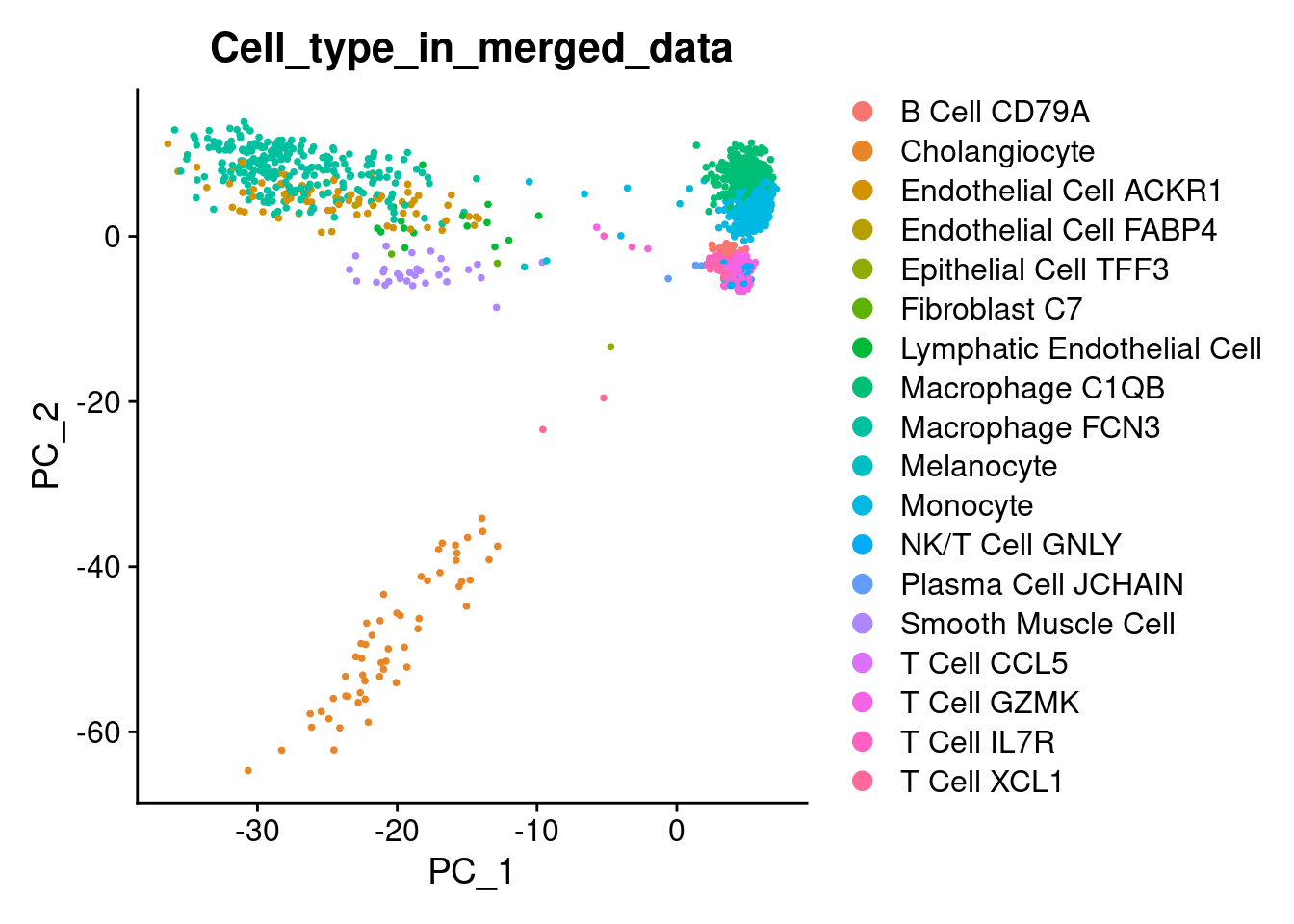
Plot PCA
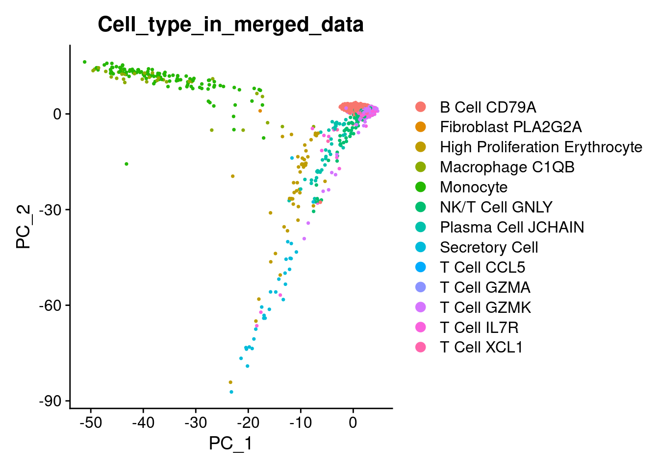
1DimPlot(liver, reduction = "pca", group.by = 'Cell_type_in_merged_data')
Plot UMAP
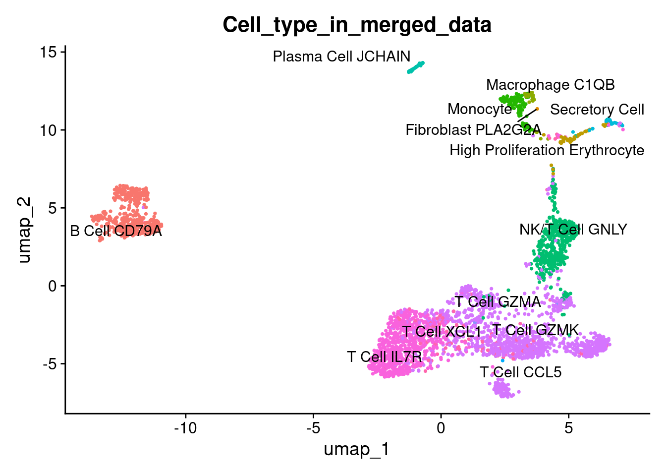
1DimPlot(liver, reduction = "umap", label = TRUE, repel = TRUE, group.by = 'Cell_type_in_merged_data' ) + NoLegend()
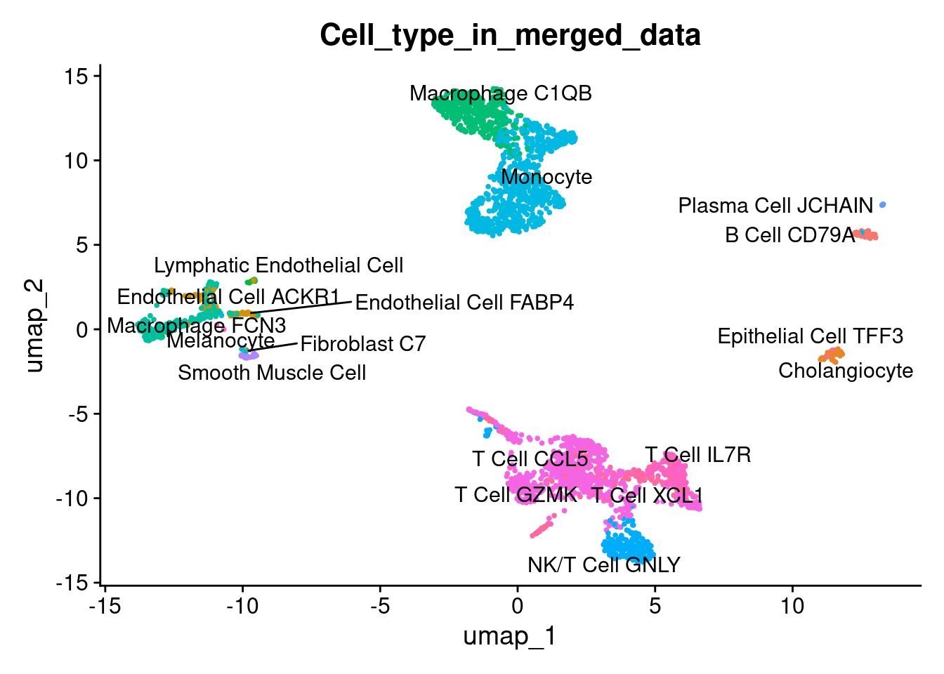
Plot PaCMAP
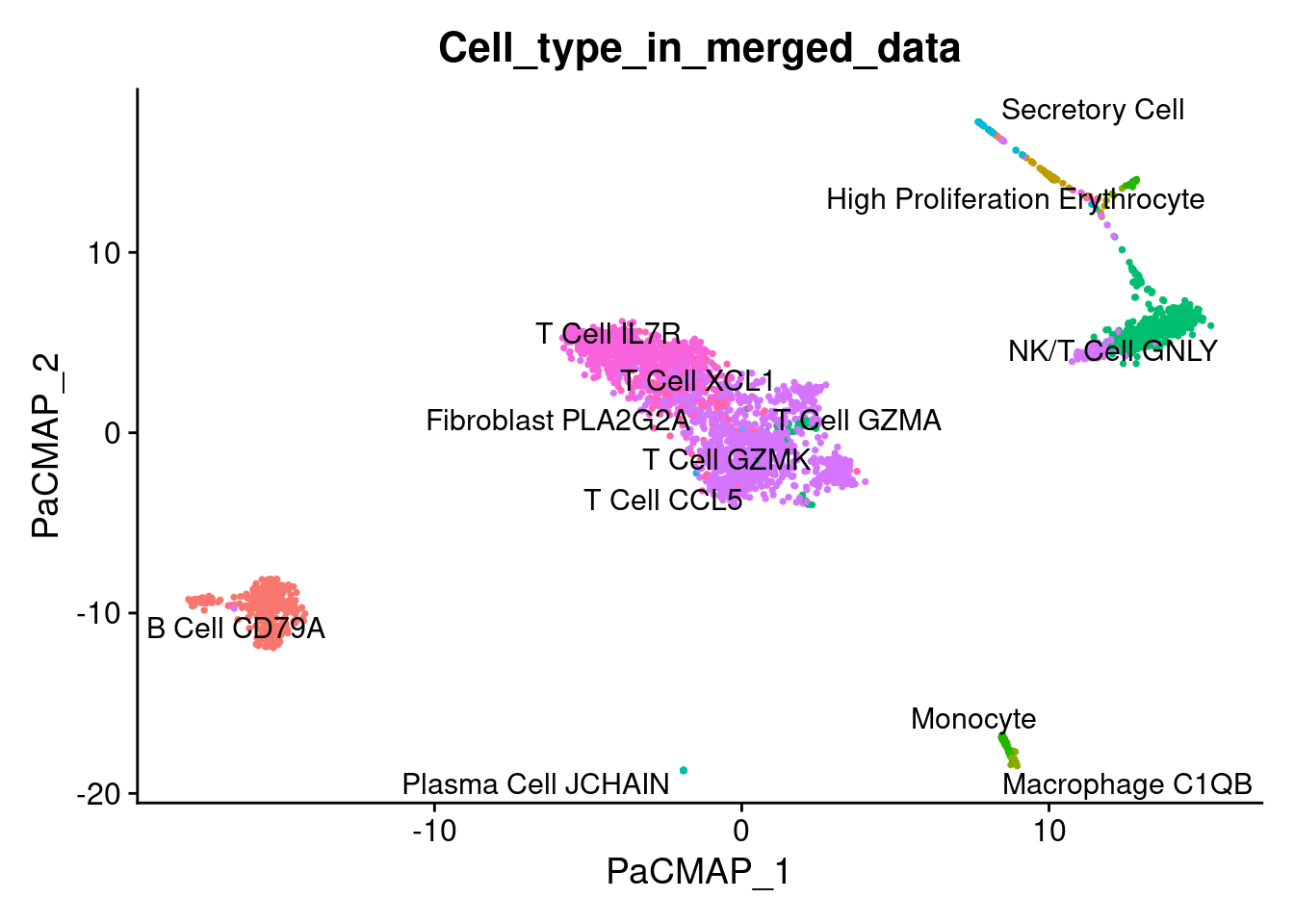
1DimPlot(liver, reduction = "pacmap", label = TRUE, repel = TRUE, group.by = 'Cell_type_in_merged_data' ) + NoLegend()

Bone Marrow
Download and normalize
1sce.marrow <- fetchDataset("he-organs-2020","2023-12-21","marrow")
2sce.marrow <- normalizeSCE(sce.marrow)
Prepare the object defining the format of the data to avoid issues converting the object.
1library(Matrix)
2counts(sce.marrow) <- as(counts(sce.marrow), "dgCMatrix")
3logcounts(sce.marrow) <- as(logcounts(sce.marrow), "dgCMatrix")
1marrow <- as.Seurat(sce.marrow, counts = "counts", data = "logcounts")
2marrow <- RenameAssays(marrow, originalexp = "RNA")
1## Renaming default assay from originalexp to RNA
1## Warning: Key 'originalexp_' taken, using 'rna_' instead
1DefaultAssay(marrow) <- "RNA"
Process using custom function
1marrow <- seuratProcessing(marrow)
1## Centering and scaling data matrix
 1## PC_ 1
 2## Positive:  CCL4, RPS6, RP11-291B21.2, PRDM1, XCL2, CD27, GZMB, LEF1, RGS1, XCL1
 3## 	   CD40LG, RPLP0, TRGV9, CCL4L2, RPS2, RPS8, FGFBP2, TRGV8, PIM2, FKBP11
 4## 	   ERN1, RPL7A, MIF, TRGV2, CXCR6, GNLY, ITGA6, CLIC3, CCR7, TRGV10
 5## Negative:  CST3, FCN1, SERPINA1, CD68, IFI30, AIF1, CD14, TMEM176B, MAFB, LST1
 6## 	   SPI1, CSF1R, MS4A7, LILRA5, LYZ, CYBB, LILRB2, IGSF6, CD302, CFP
 7## 	   LRRC25, MS4A6A, LINC01272, PILRA, DMXL2, CPVL, CFD, FTL, SLC7A7, MPEG1
 8## PC_ 2
 9## Positive:  CD68, SERPINA1, CTSS, MS4A7, FCN1, IFI30, CYBB, MAFB, AIF1, LILRA5
10## 	   LST1, LILRB2, CSF1R, TMEM176B, CD14, SPI1, LINC01272, CST3, PILRA, IGSF6
11## 	   TIMP1, CFP, MPEG1, CD74, LRRC25, SLC7A7, CLEC7A, DMXL2, HMOX1, C1QA
12## Negative:  CA1, AHSP, HBB, HBA2, HBA1, HBD, HBM, SLC4A1, GYPA, CA2
13## 	   RHAG, GYPB, ALAS2, SPTA1, HMBS, HEMGN, TMEM56, SLC25A37, EPB42, CR1L
14## 	   KLF1, MKI67, SPTB, SNCA, TFRC, NUSAP1, ANK1, GYPE, RHD, CENPF
15## PC_ 3
16## Positive:  CD79A, MS4A1, HLA-DRA, BANK1, MEF2C, RALGPS2, CD74, LINC00926, FAM129C, CD79B
17## 	   POU2AF1, IGHM, IGKC, HLA-DQA1, TCF4, VPREB3, ADAM28, HLA-DQB1, MZB1, AFF3
18## 	   SPIB, RP11-693J15.5, HLA-DRB1, FCRL5, RPS8, CD22, JCHAIN, FCRLA, SYK, IGHA1
19## Negative:  CCL4, GZMB, GNLY, FCGR3A, TYROBP, FGFBP2, KLRF1, MT2A, CX3CR1, SAMHD1
20## 	   CLIC3, SPON2, CTSD, FCER1G, XCL2, TRDC, KLRC3, LGALS1, RP11-291B21.2, PRDM1
21## 	   IFITM3, CCL3, SLC4A1, SH2D1B, HBM, HBA1, GAPDH, CEBPD, HBA2, KLRC2
22## PC_ 4
23## Positive:  STMN1, TYMS, GAPDH, CNRIP1, CYTL1, KIAA0101, MYB, CDT1, TK1, TXNDC5
24## 	   CMBL, EGFL7, PRSS57, ITGA2B, GINS2, MCM10, SMIM10, MAP7, NREP, APOC1
25## 	   SOX4, SDPR, ALDH1A1, GATA2, PPIB, CDK6, RP11-620J15.3, XBP1, MCM4, CDC25A
26## Negative:  SLC4A1, MS4A1, HBM, ALAS2, HBA1, GYPA, HBA2, RHAG, SLC25A37, GYPB
27## 	   CD79A, HLA-DRA, BANK1, EPB42, LINC00926, AHSP, HEMGN, CD74, SPTA1, HBD
28## 	   CA2, CR1L, FAM129C, GYPE, TSPO2, HLA-DQA1, HLA-DRB1, HBB, RHD, TMEM56
29## PC_ 5
30## Positive:  CNRIP1, CYTL1, MYB, EGFL7, CMBL, ITGA2B, SMIM10, APOC1, SDPR, ALDH1A1
31## 	   SOX4, MAP7, RPS8, GATA2, RP11-354E11.2, NREP, RPS6, PRKAR2B, MYC, RP11-620J15.3
32## 	   CDC42BPA, ZNF521, IL1B, SLC40A1, FAM178B, PRSS57, RPS2, DPPA4, CD34, HACD1
33## Negative:  TXNDC5, JCHAIN, MZB1, TNFRSF17, DERL3, GAS6, ITM2C, IGLL5, TRIB1, HSP90B1
34## 	   IGKC, XBP1, SEC11C, RRM2, ELL2, SDF2L1, MYDGF, FKBP11, PPIB, RRBP1
35## 	   IGHG1, BMP8B, PRDX4, POU2AF1, PDIA4, FNDC3B, SPCS3, IGHA1, IRF4, SSR3
1## 17:14:29 UMAP embedding parameters a = 0.9922 b = 1.112
1## 17:14:29 Read 3230 rows and found 50 numeric columns
1## 17:14:29 Using Annoy for neighbor search, n_neighbors = 30
1## 17:14:29 Building Annoy index with metric = cosine, n_trees = 50
1## 0% 10 20 30 40 50 60 70 80 90 100%
1## [----|----|----|----|----|----|----|----|----|----|
1## **************************************************|
2## 17:14:29 Writing NN index file to temp file /tmp/RtmpRhKGc1/file14a1d668374e00
3## 17:14:29 Searching Annoy index using 1 thread, search_k = 3000
4## 17:14:30 Annoy recall = 100%
5## 17:14:30 Commencing smooth kNN distance calibration using 1 thread with target n_neighbors = 30
6## 17:14:31 Initializing from normalized Laplacian + noise (using RSpectra)
7## 17:14:31 Commencing optimization for 500 epochs, with 141670 positive edges
8## 17:14:31 Using rng type: pcg
9## 17:14:34 Optimization finished
 1## Applied PCA, the dimensionality becomes 100
 2## PaCMAP(n_neighbors=10, n_MN=5, n_FP=20, distance=euclidean, lr=1.0, n_iters=(100, 100, 250), apply_pca=True, opt_method='adam', verbose=True, intermediate=False, seed=11)
 3## Finding pairs
 4## Found nearest neighbor
 5## Calculated sigma
 6## Found scaled dist
 7## Pairs sampled successfully.
 8## ((32300, 2), (16150, 2), (64600, 2))
 9## Initial Loss: 39786.1015625
10## Iteration:   10, Loss: 31564.384766
11## Iteration:   20, Loss: 26498.765625
12## Iteration:   30, Loss: 24599.064453
13## Iteration:   40, Loss: 23357.765625
14## Iteration:   50, Loss: 22296.308594
15## Iteration:   60, Loss: 21254.789062
16## Iteration:   70, Loss: 20105.675781
17## Iteration:   80, Loss: 18757.550781
18## Iteration:   90, Loss: 17056.492188
19## Iteration:  100, Loss: 14561.528320
20## Iteration:  110, Loss: 18082.763672
21## Iteration:  120, Loss: 17965.183594
22## Iteration:  130, Loss: 17916.142578
23## Iteration:  140, Loss: 17902.347656
24## Iteration:  150, Loss: 17892.806641
25## Iteration:  160, Loss: 17889.906250
26## Iteration:  170, Loss: 17887.958984
27## Iteration:  180, Loss: 17886.531250
28## Iteration:  190, Loss: 17885.644531
29## Iteration:  200, Loss: 17885.613281
30## Iteration:  210, Loss: 8883.780273
31## Iteration:  220, Loss: 8748.736328
32## Iteration:  230, Loss: 8681.777344
33## Iteration:  240, Loss: 8642.035156
34## Iteration:  250, Loss: 8625.769531
35## Iteration:  260, Loss: 8614.654297
36## Iteration:  270, Loss: 8606.169922
37## Iteration:  280, Loss: 8599.128906
38## Iteration:  290, Loss: 8592.977539
39## Iteration:  300, Loss: 8587.457031
40## Iteration:  310, Loss: 8582.447266
41## Iteration:  320, Loss: 8577.856445
42## Iteration:  330, Loss: 8573.578125
43## Iteration:  340, Loss: 8569.664062
44## Iteration:  350, Loss: 8565.967773
45## Iteration:  360, Loss: 8562.587891
46## Iteration:  370, Loss: 8559.376953
47## Iteration:  380, Loss: 8556.396484
48## Iteration:  390, Loss: 8553.584961
49## Iteration:  400, Loss: 8550.892578
50## Iteration:  410, Loss: 8548.406250
51## Iteration:  420, Loss: 8546.052734
52## Iteration:  430, Loss: 8543.774414
53## Iteration:  440, Loss: 8541.660156
54## Iteration:  450, Loss: 8539.642578
55## Elapsed time: 0.68s
plot PCA
1DimPlot(marrow, reduction = "pca", group.by = 'Cell_type_in_merged_data')
UMAP
1DimPlot(marrow, reduction = "umap", label = TRUE, repel = TRUE, group.by = 'Cell_type_in_merged_data' ) + NoLegend()
PaCMAP
1DimPlot(marrow, reduction = "pacmap", label = TRUE, repel = TRUE, group.by = 'Cell_type_in_merged_data' ) + NoLegend()
Conclusions
- Main cell type relationship does not change between PaCMAP and UMAP
- The only difference between PaCMAP and UMAP is the location of cell type clusters with very small number of cells
Take away
- I think I will include PaCMAP in my future single cell analysis, it is fast and easy to use.
- It would be interesting to compare with UMAP in a real life test
Further reading
- Towards a comprehensive evaluation of dimension reduction methods for transcriptomic data visualization -Understanding How Dimension Reduction Tools Work: An Empirical Approach to Deciphering t-SNE, UMAP, TriMap, and PaCMAP for Data Visualization
- PaCMAP github
- PaCMAP tutorial
- Reticulate
Bonus I: Animated GIF
Code to generate the GIF
 1library(magick)
 2
 3umap_plot <- DimPlot(marrow, reduction = "umap", label = TRUE, repel = TRUE, group.by = 'Cell_type_in_merged_data') +
 4  ggtitle("UMAP") + NoLegend()
 5
 6pacmap_plot <- DimPlot(marrow, reduction = "pacmap", label = TRUE, repel = TRUE, group.by = 'Cell_type_in_merged_data') +
 7  ggtitle("PaCMAP") + NoLegend()
 8
 9umap_plot_file <- tempfile(fileext = ".png")
10pacmap_plot_file <- tempfile(fileext = ".png")
11ggsave(umap_plot_file, plot = umap_plot, width = 6, height = 6)
12ggsave(pacmap_plot_file, plot = pacmap_plot, width = 6, height = 6)
13
14umap_img <- image_read(umap_plot_file)
15pacmap_img <- image_read(pacmap_plot_file)
16
17frames <- c(umap_img, pacmap_img)
18gif <- image_animate(image_join(frames), fps = 1)
19
20image_write(gif, "UMAP_PaCMAP.gif")
Bonus II: Code solution
Here the code I used for the two extra datasets.
 1normalizeSCE <- function(sce) {
 2  require(scran)
 3  sce.clusters <- quickCluster(sce, BPPARAM=BiocParallel::MulticoreParam(8))
 4  sce <- computeSumFactors( sce,
 5                            cluster=sce.clusters,
 6                            min.mean=0.1,
 7                            BPPARAM=BiocParallel::MulticoreParam(8)
 8                          )
 9  sce <- logNormCounts( sce, BPPARAM=BiocParallel::MulticoreParam(8) )
10  return(sce)
11}
12
13seuratProcessing <- function(seurat){
14  seurat <- FindVariableFeatures( seurat, selection.method = "vst", nfeatures = 2000) %>%
15    ScaleData( features = rownames(.) ) %>%
16    RunPCA( features = VariableFeatures(object = .)) %>%
17    RunUMAP( dims = 1:50) %>%
18    RunPaCMAP(features = Seurat::VariableFeatures(.))
19 return(seurat)
20}