Alignment or Pseudoalignment: Alevin-fry vs Cell Ranger comparison
Last week post explained how to use simpleaf to run alevin-fry on a single cell RNA-seq dataset. This post will compare the results of alevin-fry with those of cellranger, the official 10x Genomics pipeline for single cell RNA-seq data analysis.
Let's start by checking the knee plot from the Cell Ranger html report.
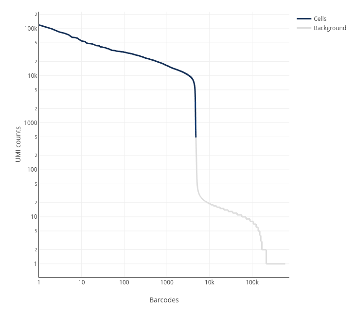
Now we can download Cell Ranger results from the 5k Human PBMCs (Donor 3) dataset website, this way we do not need to run Cell Ranger ourselves. We will use the filtered matrix, which is the result of selecting the cells labeled in blue in the knee plot.
1wget https://cf.10xgenomics.com/samples/cell-exp/9.0.0/5k_Human_Donor3_PBMC_3p_gem-x_5k_Human_Donor3_PBMC_3p_gem-x/5k_Human_Donor3_PBMC_3p_gem-x_5k_Human_Donor3_PBMC_3p_gem-x_count_sample_filtered_feature_bc_matrix.tar.gz
2tar -xvzf 5k_Human_Donor3_PBMC_3p_gem-x_5k_Human_Donor3_PBMC_3p_gem-x_count_sample_filtered_feature_bc_matrix.tar.gz
Next step is to read the files and create a SingleCellExperiment (SCE) object. If you are not familiar with SCE objects, take a look to my post Single cell Bioconductor's choice: SCE.
First we set variables
1matrix_dir_filtered <- 'sample_filtered_feature_bc_matrix'
2features.path <- paste0(matrix_dir_filtered, "/features.tsv.gz")
3barcodes.path <- paste0(matrix_dir_filtered, "/barcodes.tsv.gz")
4matrix.path <- paste0(matrix_dir_filtered, "/matrix.mtx.gz")
and then read the files to create the SCE object
 1library( Matrix )
 2library( SingleCellExperiment )
 3mat <- readMM(file = matrix.path)
 4feature.names = read.delim(features.path,
 5                           header = FALSE,
 6                           stringsAsFactors = FALSE)
 7barcode.names = read.delim(barcodes.path,
 8                           header = FALSE,
 9                           stringsAsFactors = FALSE)
10colnames(mat) = barcode.names$V1
11rownames(mat) = feature.names$V1
12mat <- mat[ rowSums(mat) != 0, ]
13sce.cellranger <- SingleCellExperiment( assays = list( counts = mat ) )
check object
1sce.cellranger
 1## class: SingleCellExperiment
 2## dim: 27439 4782
 3## metadata(0):
 4## assays(1): counts
 5## rownames(27439): ENSG00000238009 ENSG00000239945 ... ENSG00000275063
 6##   ENSG00000278817
 7## rowData names(0):
 8## colnames(4782): AAACCAAAGCGCCTTC-1 AAACCAAAGTTAATGC-1 ...
 9##   TGTGTTGAGCTTAGTG-1 TGTGTTGAGGAATGAC-1
10## colData names(0):
11## reducedDimNames(0):
12## mainExpName: NULL
13## altExpNames(0):
Now we can load the alevin-fry resulst using the fishpond R package as in my last post.
1myPath<- '/media/alfonso/data/nextflow_PBMCs/output/quant/pbmc5k_d3_quant/af_quant/'
2
3custom_format <- list("counts" = c("U", "S", "A"),
4                      "spliced" = c("S"),
5                      "unspliced" = c("U"),
6                      "ambiguous" = c("A"))
7sce.alevin <- fishpond::loadFry(myPath,
8                         outputFormat = custom_format)
1## locating quant file
1## Reading meta data
1## USA mode: TRUE
1## Processing 38606 genes and 157273 barcodes
1## Using user-defined output assays
1## Building the 'counts' assay, which contains U S A
1## Building the 'spliced' assay, which contains S
1## Building the 'unspliced' assay, which contains U
1## Building the 'ambiguous' assay, which contains A
1## Constructing output SingleCellExperiment object
1## Done
as we know, this object is not filtered. Let's filter it using the DropletUtils package.
1library(DropletUtils)
2bcrank <- barcodeRanks(counts(sce.alevin))
let's explore the results with a kneeplot
1uniq <- !duplicated(bcrank$rank)
2plot(bcrank$rank[uniq], bcrank$total[uniq], log="xy",
3    xlab="Rank", ylab="Total UMI count", cex.lab=1.2)
4abline(h=metadata(bcrank)$inflection, col="darkgreen", lty=2)
5abline(h=metadata(bcrank)$knee, col="dodgerblue", lty=2)
6legend("bottomleft", legend=c("Inflection", "Knee"),
7        col=c("darkgreen", "dodgerblue"), lty=2, cex=1.2)
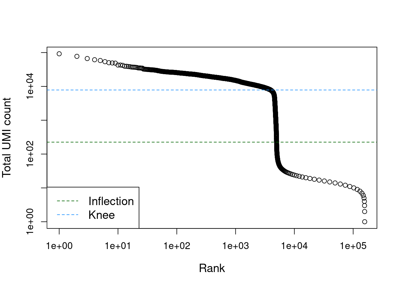
Now we can filter the alevin-fry object using the inflection point calculated by barcodeRanks function, we use the inflection point as it seems closer to the Cell Ranger's knee plot cell selection.
1sce.alevin <- sce.alevin[, bcrank$total >= metadata(bcrank)$inflection]
2sce.alevin <- sce.alevin[ rowSums(counts(sce.alevin)) > 0, ]
3sce.alevin
 1## class: SingleCellExperiment
 2## dim: 27249 4986
 3## metadata(0):
 4## assays(4): counts spliced unspliced ambiguous
 5## rownames(27249): ENSG00000274847 ENSG00000278384 ... ENSG00000286130
 6##   ENSG00000290841
 7## rowData names(1): gene_ids
 8## colnames(4986): ATCCCGCTCGTGCCCT TGAAACGGTTAACGCT ... TCGCTCTGTTGCACCA
 9##   TGAGTAGGTGGCAGTG
10## colData names(1): barcodes
11## reducedDimNames(0):
12## mainExpName: NULL
13## altExpNames(0):
From the dimensions of both SCE objects, we can see that both objects have close to 5000 cells. However, the Cell Ranger object has around 4700 while the alevin-fry around 4900.
We use a Venn diagram to compare the cells in both objects
 1library(VennDiagram)
 2library(wesanderson)
 3
 4cells.list <- list( cellranger = gsub( '-1', '', colnames(sce.cellranger) ),
 5                    alevinfry = colnames(sce.alevin)
 6                  )
 7
 8venn.diagram( cells.list,
 9              "Venn.diagram.tiff",
10              fill=wes_palette("FantasticFox1")[1:length(cells.list)],
11              alpha=rep( 0.25, length(cells.list) ),
12              cex = 2.5, cat.fontface=4,
13              category.names = names(cells.list),
14              col=wes_palette("FantasticFox1")[1:length(cells.list)]
15            )
16
17cmd <- 'convert Venn.diagram.tiff Venn.diagram.png && rm Venn.diagram.tiff '
18system( cmd )
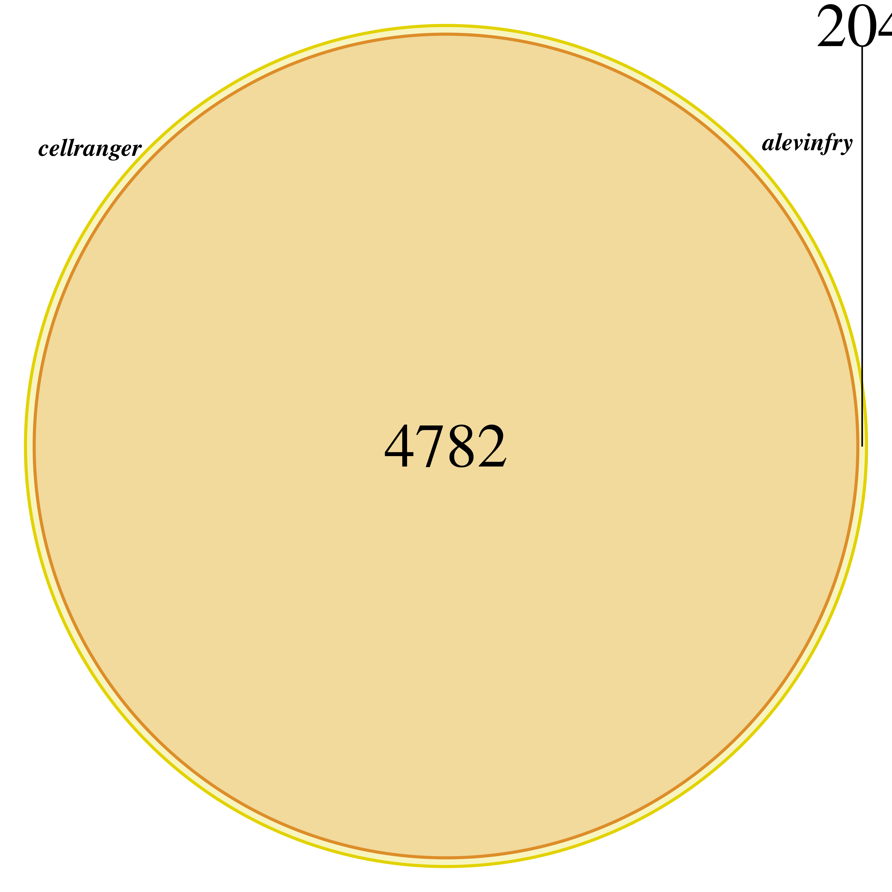
We see that all cells detected by Cell Ranger are also detected by alevin-fry, with alevin-fry detecting a few more.
This is most likely due to the barcodeRanks function's inflection point definition. In any case, this is not highly relevant as the first step recommended in any single cell workflow is filtering low quality cells using number of detected genes, number of UMIs, and percentage of mitochondrial genes.
Now we check the detected genes by each method.
 1cells.list <- list( cellranger = rownames(sce.cellranger),
 2                    alevinfry = rownames(sce.alevin)
 3                  )
 4
 5venn.diagram( cells.list,
 6              "Venn.rownames.tiff",
 7              fill=wes_palette("FantasticFox1")[1:length(cells.list)],
 8              alpha=rep( 0.25, length(cells.list) ),
 9              cex = 2.5, cat.fontface=4,
10              category.names = names(cells.list),
11              col=wes_palette("FantasticFox1")[1:length(cells.list)]
12            )
13
14cmd <- 'convert Venn.rownames.tiff Venn.rownames.png && rm Venn.rownames.tiff '
15system( cmd )
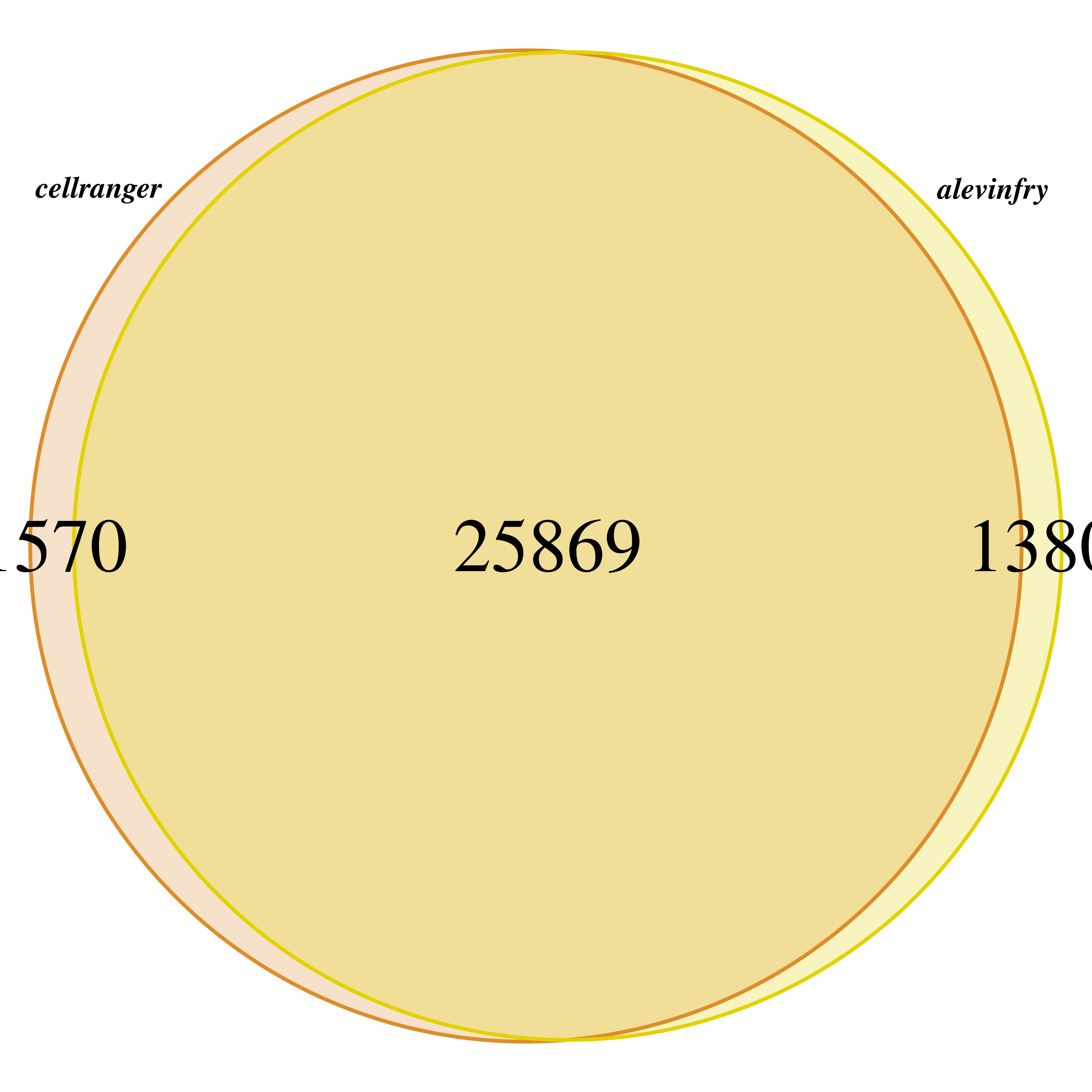
Again, very similar resuts, with over 25000 genes in common and only a little over 1000 genes detected specifically by one method.
Let's compare the expression in both methods with a scatter plot. In this plot each dot is the gene expression of a gene in a cell.
1library(ggplot2)
2library(dplyr)
1##
2## Attaching package: 'dplyr'
1## The following object is masked from 'package:Biobase':
2##
3##     combine
1## The following objects are masked from 'package:GenomicRanges':
2##
3##     intersect, setdiff, union
1## The following object is masked from 'package:GenomeInfoDb':
2##
3##     intersect
1## The following objects are masked from 'package:IRanges':
2##
3##     collapse, desc, intersect, setdiff, slice, union
1## The following objects are masked from 'package:S4Vectors':
2##
3##     first, intersect, rename, setdiff, setequal, union
1## The following objects are masked from 'package:BiocGenerics':
2##
3##     combine, intersect, setdiff, union
1## The following object is masked from 'package:matrixStats':
2##
3##     count
1## The following objects are masked from 'package:stats':
2##
3##     filter, lag
1## The following objects are masked from 'package:base':
2##
3##     intersect, setdiff, setequal, union
1library(tidyr)
1##
2## Attaching package: 'tidyr'
1## The following object is masked from 'package:S4Vectors':
2##
3##     expand
1## The following objects are masked from 'package:Matrix':
2##
3##     expand, pack, unpack
 1cr.counts.df <- counts(sce.cellranger) %>%
 2  as.matrix() %>%
 3  as.data.frame() %>%
 4  tibble::rownames_to_column(var = "gene") %>%
 5  pivot_longer(-gene, names_to = "cell", values_to = "cellranger") %>%
 6  mutate(cell = gsub( '-1', '', cell ))
 7
 8alevin.counts.df <- counts(sce.alevin) %>%
 9  as.matrix() %>%
10  as.data.frame() %>%
11  tibble::rownames_to_column(var = "gene") %>%
12  pivot_longer(-gene, names_to = "cell", values_to = "alevin")
1## Warning in asMethod(object): sparse->dense coercion: allocating vector of size
2## 1.0 GiB
 1plot.df <- cr.counts.df %>%
 2  full_join(alevin.counts.df, by = c("gene", "cell")) %>%
 3  replace_na(list(alevin = 0, cellranger = 0)) %>%
 4  filter( !( cellranger == 0 & alevin == 0 ) )
 5
 6ggplot(plot.df, aes(x = cellranger, y = alevin)) +
 7  geom_abline(slope = 1, intercept = 0, color = "navy") +
 8  geom_point(alpha = 0.1) +
 9  # scale_x_log10() +
10  # scale_y_log10() +
11  labs(x = "Cell Ranger Counts", y = "Alevin-Fry Counts") +
12  theme_bw() +
13  theme(legend.position = "none")
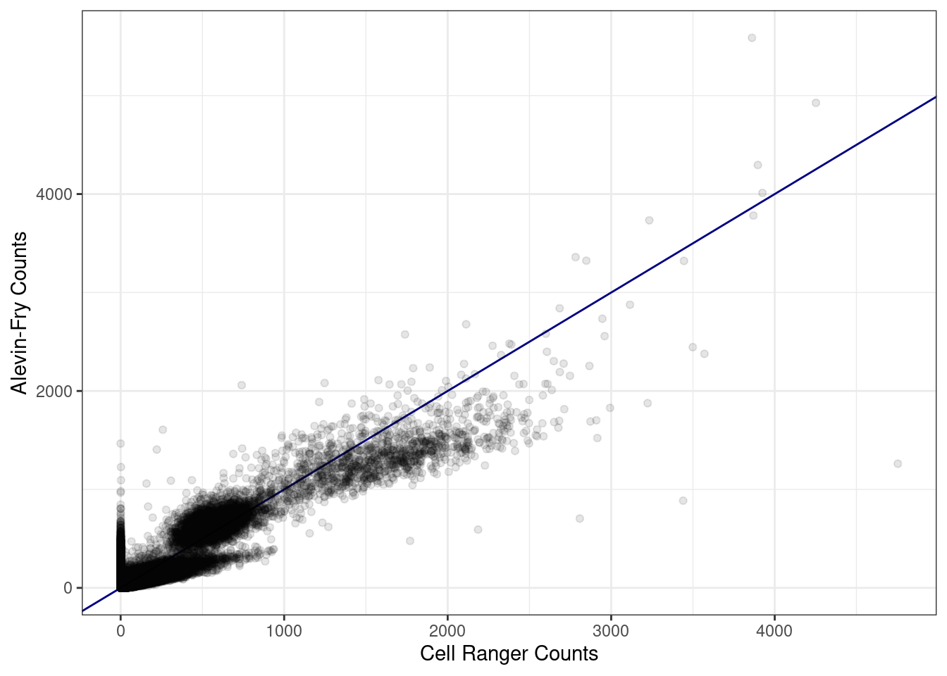
In general, most genes are detected at 'comparable' levels by both methods. We already knew from the Venn diagram analysis that a little over 1000 genes were only detected by one of the methods. The scatter plots shows that the genes only detected by alevin-fry have a significant expression, that's why we see that column of cells at x = 0.
We start by quantifying genes that not detected by cellranger but detected by alevin-fry.
1plot.df %>%
2  filter( cellranger == 0 & alevin > 0 ) %>%
3  select(gene) %>%
4  distinct() %>%
5  nrow()
1## [1] 26694
most genes are detected in at least one cell by alevin-fry but not cellranger. This is quite expected due to the known dropout effect in single cell RNAseq.
Let's try to quantify the number of cells per gene.
1summary <- plot.df %>%
2  filter( cellranger == 0 & alevin > 0 ) %>%
3  group_by(gene) %>%
4  summarise( n_cells = n(), max = max(alevin), avg = mean(alevin), median = median(alevin), min = min(alevin) )
Let's take a look to the genes detected in the higher number of cells.
1summary %>%
2  arrange(desc(n_cells)) %>%
3  head(20)
 1## # A tibble: 20 × 6
 2##    gene            n_cells   max    avg median   min
 3##    <chr>             <int> <dbl>  <dbl>  <dbl> <dbl>
 4##  1 ENSG00000101333    4931    90  12.3      11     1
 5##  2 ENSG00000247134    4769    51   8.55      8     1
 6##  3 ENSG00000228716    4718  1466 220.      203     1
 7##  4 ENSG00000178568    4410    21   3.10      3     1
 8##  5 ENSG00000280441    4366   427  68.0      60     1
 9##  6 ENSG00000163590    4005   123  18.9      18     1
10##  7 ENSG00000211592    3887    12   2.71      2     1
11##  8 ENSG00000125538    3684    33   3.56      3     1
12##  9 ENSG00000163220    3588    63   6.79      6     1
13## 10 ENSG00000038427    3577    38   4.39      4     1
14## 11 ENSG00000169429    3559    20   3.26      3     1
15## 12 ENSG00000236383    3513    31   2.75      2     1
16## 13 ENSG00000090382    3502   148  16.9      16     1
17## 14 ENSG00000123689    3479    30   3.93      3     1
18## 15 ENSG00000101439    3478    41   5.10      5     1
19## 16 ENSG00000153823    3390    24   3.11      3     1
20## 17 ENSG00000143546    3369    17   2.98      3     1
21## 18 ENSG00000085265    3353    24   3.30      3     1
22## 19 ENSG00000211899    3342    10   2.04      2     1
23## 20 ENSG00000124882    3310    22   2.75      2     1
Now let's focus on those genes with highest averagte expression.
1summary %>%
2  arrange(desc(avg)) %>%
3  head(20)
 1## # A tibble: 20 × 6
 2##    gene            n_cells   max   avg median   min
 3##    <chr>             <int> <dbl> <dbl>  <dbl> <dbl>
 4##  1 ENSG00000228716    4718  1466 220.     203     1
 5##  2 ENSG00000280441    4366   427  68.0     60     1
 6##  3 ENSG00000251562     216   619  57.3     45     8
 7##  4 ENSG00000163590    4005   123  18.9     18     1
 8##  5 ENSG00000090382    3502   148  16.9     16     1
 9##  6 ENSG00000167996     363    83  16.1     10     1
10##  7 ENSG00000133112     387   198  15.7     10     1
11##  8 ENSG00000137818     383   144  15.0      8     1
12##  9 ENSG00000156508     316   162  14.8      9     1
13## 10 ENSG00000198804     205    53  14.6     13     1
14## 11 ENSG00000167526     362   104  14.2      8     1
15## 12 ENSG00000142937     401   111  13.9      8     1
16## 13 ENSG00000147403     396   126  13.7      8     1
17## 14 ENSG00000112306     425    87  13.2      7     1
18## 15 ENSG00000101333    4931    90  12.3     11     1
19## 16 ENSG00000142541     399   109  11.7      7     1
20## 17 ENSG00000164587     456    96  11.6      7     1
21## 18 ENSG00000019582    1173    32  11.6     12     1
22## 19 ENSG00000145425     387   104  11.2      6     1
23## 20 ENSG00000169554    2395    41  11.2     11     1
Checking a few of the genes detected in most cells at significant levels, we find:
- ENSG00000228716, a dihydrofolate reductase whose deficiency has been linked to megaloblastic anemia. Several transcript variants encoding different isoforms have been found for this gene.
- ENSG00000280441, a lncRNA with little information available.
- ENSG00000163590, a magnesium or manganese-requiring phosphatase that is involved in several signaling pathways
it would be interesting to check if gene detected in lower number of cells are associated with specific cell types or clusters.
Conclusions
- Both methods produce similar results.
- It would be interesting to evaluate the expression of 'method specific' genes, specially in the context of cell type or cluster specific expression.
- It would also be interesting to check if these minor differences have an effect on downstream analyses.
Further reading
- 10X Genomics: Cell Ranger
- "Single-cell best practices" book: Quality Control
- “Orchestrating Single-Cell Analysis with Bioconductor” book: Chapter 1 Quality Control
- Seurat - Guided Clustering Tutorial: QC and selecting cells for further analy