Autoencoders for Single Cell Data Analysis
We live in the age of AI, machine learning, deep learning and LLMs. Today we will focus in autoencoders.
Autoencoders can be defined as a class of unsupervised neural networks designed to learn compact, informative representations of data by encoding inputs into a low-dimensional latent space and then reconstructing them. I see autoencoders as the deep learning version of PCA.
1##
2## Attaching package: 'dplyr'
1## The following objects are masked from 'package:stats':
2##
3##     filter, lag
1## The following objects are masked from 'package:base':
2##
3##     intersect, setdiff, setequal, union
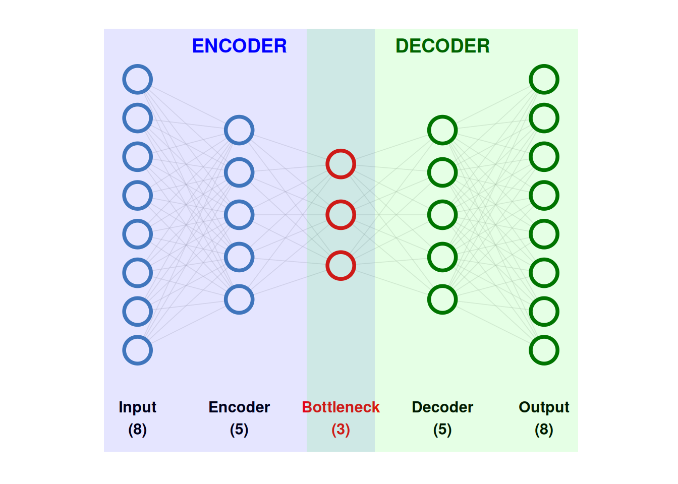
These are the basic components of an autoencoder:
- Input layer: Receives the original data and passes it to the network for encoding.
- Encoder: Transforms the input data into a lower-dimensional representation by learning informative features.
- Latent space (bottleneck): A compressed representation that captures the most salient information needed to reconstruct the input.
- Decoder: Maps the latent representation back to the original data space.
- Output (reconstruction): The network’s attempt to reproduce the original input as accurately as possible.
In single-cell, autoencoders can be used to model the high dimensionality, sparsity, and technical noise inherent in single-cell RNA-sequencing data. For example, scVI (single-cell variational inference) uses a variational autoencoder framework to perform batch correction, dimensionality reduction, and probabilistic modeling of gene expression, while methods like DCA (Deep Count Autoencoder) focus on denoising and handling dropout events, and SAUCIE uses autoencoders for visualization, clustering, and batch effect removal.
we will use the pancreas dataset as in my slingshot and RNA velocity post.
1library(zellkonverter)
1## Registered S3 method overwritten by 'zellkonverter':
2##   method                                             from
3##   py_to_r.pandas.core.arrays.categorical.Categorical reticulate
1sce <- readH5AD( file.path( data.path, 'endocrinogenesis_day15.h5ad' ) )
1sce
 1## class: SingleCellExperiment
 2## dim: 27998 3696
 3## metadata(5): clusters_coarse_colors clusters_colors day_colors
 4##   neighbors pca
 5## assays(3): X spliced unspliced
 6## rownames(27998): Xkr4 Gm37381 ... Gm20837 Erdr1
 7## rowData names(1): highly_variable_genes
 8## colnames(3696): AAACCTGAGAGGGATA AAACCTGAGCCTTGAT ... TTTGTCATCGAATGCT
 9##   TTTGTCATCTGTTTGT
10## colData names(4): clusters_coarse clusters S_score G2M_score
11## reducedDimNames(2): X_pca X_umap
12## mainExpName: NULL
13## altExpNames(0):
save X assay as logcounts to make our life easier.
1library(SingleCellExperiment)
1## Loading required package: SummarizedExperiment
1## Loading required package: MatrixGenerics
1## Loading required package: matrixStats
1##
2## Attaching package: 'matrixStats'
1## The following object is masked from 'package:dplyr':
2##
3##     count
1##
2## Attaching package: 'MatrixGenerics'
 1## The following objects are masked from 'package:matrixStats':
 2##
 3##     colAlls, colAnyNAs, colAnys, colAvgsPerRowSet, colCollapse,
 4##     colCounts, colCummaxs, colCummins, colCumprods, colCumsums,
 5##     colDiffs, colIQRDiffs, colIQRs, colLogSumExps, colMadDiffs,
 6##     colMads, colMaxs, colMeans2, colMedians, colMins, colOrderStats,
 7##     colProds, colQuantiles, colRanges, colRanks, colSdDiffs, colSds,
 8##     colSums2, colTabulates, colVarDiffs, colVars, colWeightedMads,
 9##     colWeightedMeans, colWeightedMedians, colWeightedSds,
10##     colWeightedVars, rowAlls, rowAnyNAs, rowAnys, rowAvgsPerColSet,
11##     rowCollapse, rowCounts, rowCummaxs, rowCummins, rowCumprods,
12##     rowCumsums, rowDiffs, rowIQRDiffs, rowIQRs, rowLogSumExps,
13##     rowMadDiffs, rowMads, rowMaxs, rowMeans2, rowMedians, rowMins,
14##     rowOrderStats, rowProds, rowQuantiles, rowRanges, rowRanks,
15##     rowSdDiffs, rowSds, rowSums2, rowTabulates, rowVarDiffs, rowVars,
16##     rowWeightedMads, rowWeightedMeans, rowWeightedMedians,
17##     rowWeightedSds, rowWeightedVars
1## Loading required package: GenomicRanges
1## Loading required package: stats4
1## Loading required package: BiocGenerics
1##
2## Attaching package: 'BiocGenerics'
1## The following objects are masked from 'package:dplyr':
2##
3##     combine, intersect, setdiff, union
1## The following objects are masked from 'package:stats':
2##
3##     IQR, mad, sd, var, xtabs
1## The following objects are masked from 'package:base':
2##
3##     anyDuplicated, aperm, append, as.data.frame, basename, cbind,
4##     colnames, dirname, do.call, duplicated, eval, evalq, Filter, Find,
5##     get, grep, grepl, intersect, is.unsorted, lapply, Map, mapply,
6##     match, mget, order, paste, pmax, pmax.int, pmin, pmin.int,
7##     Position, rank, rbind, Reduce, rownames, sapply, setdiff, table,
8##     tapply, union, unique, unsplit, which.max, which.min
1## Loading required package: S4Vectors
1##
2## Attaching package: 'S4Vectors'
1## The following objects are masked from 'package:dplyr':
2##
3##     first, rename
1## The following object is masked from 'package:utils':
2##
3##     findMatches
1## The following objects are masked from 'package:base':
2##
3##     expand.grid, I, unname
1## Loading required package: IRanges
1##
2## Attaching package: 'IRanges'
1## The following objects are masked from 'package:dplyr':
2##
3##     collapse, desc, slice
1## Loading required package: GenomeInfoDb
1## Loading required package: Biobase
1## Welcome to Bioconductor
2##
3##     Vignettes contain introductory material; view with
4##     'browseVignettes()'. To cite Bioconductor, see
5##     'citation("Biobase")', and for packages 'citation("pkgname")'.
1##
2## Attaching package: 'Biobase'
1## The following object is masked from 'package:MatrixGenerics':
2##
3##     rowMedians
1## The following objects are masked from 'package:matrixStats':
2##
3##     anyMissing, rowMedians
1logcounts( sce ) <- assay( sce, 'X' )
prep input data for neural network, to speed up computations we will work with the 2000 most variable genes.
1library(scran)
1## Loading required package: scuttle
1dec <- modelGeneVar(sce)
1## Warning in regularize.values(x, y, ties, missing(ties), na.rm = na.rm):
2## collapsing to unique 'x' values
1hvg.pbmc.var <- getTopHVGs(dec, n=2000)
2hvg.mat <- logcounts(sce)[hvg.pbmc.var,]
3write.csv( as.matrix(hvg.mat), 'hgv.genes.mat.csv' )
to use tensorflow, the easiest way is to run it with docker as explained in my post.
1docker run -p 8888:8888 -v ./:/tf/autoencoder --gpus all -it --rm tensorflow/tensorflow:2.15.0-gpu-jupyter
select new notebook and then run the following python code, we start importing tensorflow and required classes
1import tensorflow as tf
2from tensorflow.keras.layers import Input, Dense
3from tensorflow.keras.models import Model
12025-12-13 18:55:50.357811: E external/local_xla/xla/stream_executor/cuda/cuda_dnn.cc:9261] Unable to register cuDNN factory: Attempting to register factory for plugin cuDNN when one has already been registered
22025-12-13 18:55:50.357833: E external/local_xla/xla/stream_executor/cuda/cuda_fft.cc:607] Unable to register cuFFT factory: Attempting to register factory for plugin cuFFT when one has already been registered
32025-12-13 18:55:50.358524: E external/local_xla/xla/stream_executor/cuda/cuda_blas.cc:1515] Unable to register cuBLAS factory: Attempting to register factory for plugin cuBLAS when one has already been registered
42025-12-13 18:55:50.362622: I tensorflow/core/platform/cpu_feature_guard.cc:182] This TensorFlow binary is optimized to use available CPU instructions in performance-critical operations.
5To enable the following instructions: AVX2 FMA, in other operations, rebuild TensorFlow with the appropriate compiler flags.
now install the packages that are not included in this docker, if you are going to do this regularly just create a new image starting from this one.
1!pip install pandas numpy scikit-learn
 1Requirement already satisfied: pandas in /usr/local/lib/python3.11/dist-packages (2.3.3)
 2Requirement already satisfied: numpy in /usr/local/lib/python3.11/dist-packages (1.26.2)
 3Requirement already satisfied: scikit-learn in /usr/local/lib/python3.11/dist-packages (1.8.0)
 4Requirement already satisfied: python-dateutil>=2.8.2 in /usr/local/lib/python3.11/dist-packages (from pandas) (2.8.2)
 5Requirement already satisfied: pytz>=2020.1 in /usr/local/lib/python3.11/dist-packages (from pandas) (2025.2)
 6Requirement already satisfied: tzdata>=2022.7 in /usr/local/lib/python3.11/dist-packages (from pandas) (2025.3)
 7Requirement already satisfied: scipy>=1.10.0 in /usr/local/lib/python3.11/dist-packages (from scikit-learn) (1.16.3)
 8Requirement already satisfied: joblib>=1.3.0 in /usr/local/lib/python3.11/dist-packages (from scikit-learn) (1.5.2)
 9Requirement already satisfied: threadpoolctl>=3.2.0 in /usr/local/lib/python3.11/dist-packages (from scikit-learn) (3.6.0)
10Requirement already satisfied: six>=1.5 in /usr/lib/python3/dist-packages (from python-dateutil>=2.8.2->pandas) (1.16.0)
11[33mWARNING: Running pip as the 'root' user can result in broken permissions and conflicting behaviour with the system package manager. It is recommended to use a virtual environment instead: https://pip.pypa.io/warnings/venv[0m[33m
12[0m
13[1m[[0m[34;49mnotice[0m[1;39;49m][0m[39;49m A new release of pip is available: [0m[31;49m23.3.1[0m[39;49m -> [0m[32;49m25.3[0m
14[1m[[0m[34;49mnotice[0m[1;39;49m][0m[39;49m To update, run: [0m[32;49mpython3 -m pip install --upgrade pip[0m
import the packages
1import pandas as pd
2import numpy as np
3from sklearn.preprocessing import StandardScaler
read the gene information
1csv_file_path = 'hgv.genes.mat.csv'
2data = pd.read_csv(csv_file_path, index_col=0)
take a look to the data
1data.iloc[:5, :5]
| AAACCTGAGAGGGATA | AAACCTGAGCCTTGAT | AAACCTGAGGCAATTA | AAACCTGCATCATCCC | AAACCTGGTAAGTGGC | |
|---|---|---|---|---|---|
| Pyy | 103 | 0 | 11 | 0 | 1 |
| Ghrl | 0 | 1 | 0 | 0 | 0 |
| Iapp | 0 | 0 | 27 | 0 | 0 |
| Gcg | 0 | 0 | 0 | 0 | 0 |
| Ins1 | 0 | 0 | 0 | 0 | 0 |
A common approach in 'regular' autoencoders is transforming the data with StandardScaler from sckitlearn to scale the data. However, StandardScaler is usually not recommended for scRNA-seq autoencoders.
- Log2 normalized data is is non-negative.
- Many zeros remain biologically meaningful.
- Variance across genes is informative
so we split input dat into train and test data. Instead of manual splitting, this approach shuffles the data avoiding posible Batch effects leakage and cell-type ordering bias
1from sklearn.model_selection import train_test_split
2train_data, test_data = train_test_split(input_data, test_size=0.2, random_state=42)
check the split by printing the shape (dimensions) of the resulting arrays
1print("Training data shape:", train_data.shape)
2print("Testing data shape:", test_data.shape)
1Training data shape: (2956, 2000)
2Testing data shape: (740, 2000)
It is time to configure our autoencoder. We start defining the number of neurons per layer
1neurons = [2**x for x in range(1,11)]
2neurons
1[2, 4, 8, 16, 32, 64, 128, 256, 512, 1024]
now the learning rate and the number of epochs.
The learning rate is a hyperparameter that controls how much a model's parameters are updated in response to the estimated error at each training step.
The number of epochs refers to how many complete passes the learning algorithm makes over the entire training dataset, with more epochs allowing the model to learn more.
1custom_learning_rate = 0.001
2epochs = 50
the next function will create the autoencoder
 1def create_autoencoder(neurons, input_shape):
 2    input_layer = Input(shape=(input_shape,))
 3
 4    # Encoder layers
 5    encoder_output = input_layer
 6    for i in range(len(neurons)-1, 0, -1):
 7        encoder_output = Dense(neurons[i], activation='elu')(encoder_output)
 8
 9    # Hidden layer with a name
10    hidden_layer = Dense(neurons[0], activation='linear', name='hidden_layer')(encoder_output)
11
12    # Decoder layers
13    decoder_output = hidden_layer
14    for i in range(1, len(neurons)):
15        decoder_output = Dense(neurons[i], activation='elu')(decoder_output)
16
17    # Output layer
18    output_layer = Dense(input_shape, activation='linear')(decoder_output)
19    # output_layer = Dense(input_shape, activation='sigmoid')(decoder_output) # changed because input goes from -1 to 1
20
21    autoencoder = Model(inputs=input_layer, outputs=output_layer)
22    return autoencoder
now we use it to set up our autoencoder
1autoencoder = create_autoencoder(neurons, train_data.shape[1])
 12025-12-13 19:04:48.696696: I external/local_xla/xla/stream_executor/cuda/cuda_executor.cc:901] successful NUMA node read from SysFS had negative value (-1), but there must be at least one NUMA node, so returning NUMA node zero. See more at https://github.com/torvalds/linux/blob/v6.0/Documentation/ABI/testing/sysfs-bus-pci#L344-L355
 22025-12-13 19:04:48.703243: I external/local_xla/xla/stream_executor/cuda/cuda_executor.cc:901] successful NUMA node read from SysFS had negative value (-1), but there must be at least one NUMA node, so returning NUMA node zero. See more at https://github.com/torvalds/linux/blob/v6.0/Documentation/ABI/testing/sysfs-bus-pci#L344-L355
 32025-12-13 19:04:48.706844: I external/local_xla/xla/stream_executor/cuda/cuda_executor.cc:901] successful NUMA node read from SysFS had negative value (-1), but there must be at least one NUMA node, so returning NUMA node zero. See more at https://github.com/torvalds/linux/blob/v6.0/Documentation/ABI/testing/sysfs-bus-pci#L344-L355
 42025-12-13 19:04:48.709844: I external/local_xla/xla/stream_executor/cuda/cuda_executor.cc:901] successful NUMA node read from SysFS had negative value (-1), but there must be at least one NUMA node, so returning NUMA node zero. See more at https://github.com/torvalds/linux/blob/v6.0/Documentation/ABI/testing/sysfs-bus-pci#L344-L355
 52025-12-13 19:04:48.711871: I external/local_xla/xla/stream_executor/cuda/cuda_executor.cc:901] successful NUMA node read from SysFS had negative value (-1), but there must be at least one NUMA node, so returning NUMA node zero. See more at https://github.com/torvalds/linux/blob/v6.0/Documentation/ABI/testing/sysfs-bus-pci#L344-L355
 62025-12-13 19:04:48.713724: I external/local_xla/xla/stream_executor/cuda/cuda_executor.cc:901] successful NUMA node read from SysFS had negative value (-1), but there must be at least one NUMA node, so returning NUMA node zero. See more at https://github.com/torvalds/linux/blob/v6.0/Documentation/ABI/testing/sysfs-bus-pci#L344-L355
 72025-12-13 19:04:48.834992: I external/local_xla/xla/stream_executor/cuda/cuda_executor.cc:901] successful NUMA node read from SysFS had negative value (-1), but there must be at least one NUMA node, so returning NUMA node zero. See more at https://github.com/torvalds/linux/blob/v6.0/Documentation/ABI/testing/sysfs-bus-pci#L344-L355
 82025-12-13 19:04:48.835741: I external/local_xla/xla/stream_executor/cuda/cuda_executor.cc:901] successful NUMA node read from SysFS had negative value (-1), but there must be at least one NUMA node, so returning NUMA node zero. See more at https://github.com/torvalds/linux/blob/v6.0/Documentation/ABI/testing/sysfs-bus-pci#L344-L355
 92025-12-13 19:04:48.836391: I external/local_xla/xla/stream_executor/cuda/cuda_executor.cc:901] successful NUMA node read from SysFS had negative value (-1), but there must be at least one NUMA node, so returning NUMA node zero. See more at https://github.com/torvalds/linux/blob/v6.0/Documentation/ABI/testing/sysfs-bus-pci#L344-L355
102025-12-13 19:04:48.837020: I tensorflow/core/common_runtime/gpu/gpu_device.cc:1929] Created device /job:localhost/replica:0/task:0/device:GPU:0 with 712 MB memory:  -> device: 0, name: NVIDIA GeForce RTX 2070 SUPER, pci bus id: 0000:01:00.0, compute capability: 7.5
prep the optimizer and compile the autoencoder
1optimizer = tf.keras.optimizers.Adam(learning_rate=custom_learning_rate)
2autoencoder.compile(optimizer=optimizer, loss='mean_squared_error')
show the model using summary
1autoencoder.summary()
 1Model: "model"
 2_________________________________________________________________
 3 Layer (type)                Output Shape              Param #
 4=================================================================
 5 input_1 (InputLayer)        [(None, 2000)]            0
 6
 7 dense (Dense)               (None, 1024)              2049024
 8
 9 dense_1 (Dense)             (None, 512)               524800
10
11 dense_2 (Dense)             (None, 256)               131328
12
13 dense_3 (Dense)             (None, 128)               32896
14
15 dense_4 (Dense)             (None, 64)                8256
16
17 dense_5 (Dense)             (None, 32)                2080
18
19 dense_6 (Dense)             (None, 16)                528
20
21 dense_7 (Dense)             (None, 8)                 136
22
23 dense_8 (Dense)             (None, 4)                 36
24
25 hidden_layer (Dense)        (None, 2)                 10
26
27 dense_9 (Dense)             (None, 4)                 12
28
29 dense_10 (Dense)            (None, 8)                 40
30
31 dense_11 (Dense)            (None, 16)                144
32
33 dense_12 (Dense)            (None, 32)                544
34
35 dense_13 (Dense)            (None, 64)                2112
36
37 dense_14 (Dense)            (None, 128)               8320
38
39 dense_15 (Dense)            (None, 256)               33024
40
41 dense_16 (Dense)            (None, 512)               131584
42
43 dense_17 (Dense)            (None, 1024)              525312
44
45 dense_18 (Dense)            (None, 2000)              2050000
46
47=================================================================
48Total params: 5500186 (20.98 MB)
49Trainable params: 5500186 (20.98 MB)
50Non-trainable params: 0 (0.00 Byte)
51_________________________________________________________________
time to train the autoencoder using the training data
1H = autoencoder.fit(x = train_data, y = train_data,
2                    validation_data=(test_data, test_data),
3                    batch_size = 32, epochs = epochs, verbose = 1)
  1Epoch 1/50
  2
  3
  42025-12-13 19:05:16.520701: I external/local_xla/xla/service/service.cc:168] XLA service 0x7de6e060eb90 initialized for platform CUDA (this does not guarantee that XLA will be used). Devices:
  52025-12-13 19:05:16.520721: I external/local_xla/xla/service/service.cc:176]   StreamExecutor device (0): NVIDIA GeForce RTX 2070 SUPER, Compute Capability 7.5
  62025-12-13 19:05:16.524636: I tensorflow/compiler/mlir/tensorflow/utils/dump_mlir_util.cc:269] disabling MLIR crash reproducer, set env var `MLIR_CRASH_REPRODUCER_DIRECTORY` to enable.
  72025-12-13 19:05:16.537091: I external/local_xla/xla/stream_executor/cuda/cuda_dnn.cc:454] Loaded cuDNN version 8906
  8WARNING: All log messages before absl::InitializeLog() is called are written to STDERR
  9I0000 00:00:1765652716.584968    2328 device_compiler.h:186] Compiled cluster using XLA!  This line is logged at most once for the lifetime of the process.
 10
 11
 1293/93 [==============================] - 6s 18ms/step - loss: 32.5919 - val_loss: 31.4853
 13Epoch 2/50
 1493/93 [==============================] - 2s 16ms/step - loss: 23.7953 - val_loss: 28.6923
 15Epoch 3/50
 1693/93 [==============================] - 2s 17ms/step - loss: 23.2020 - val_loss: 35.4802
 17Epoch 4/50
 1893/93 [==============================] - 1s 15ms/step - loss: 22.8094 - val_loss: 27.7426
 19Epoch 5/50
 2093/93 [==============================] - 1s 14ms/step - loss: 25.9521 - val_loss: 30.0849
 21Epoch 6/50
 2293/93 [==============================] - 1s 16ms/step - loss: 23.6428 - val_loss: 28.0149
 23Epoch 7/50
 2493/93 [==============================] - 1s 13ms/step - loss: 21.9675 - val_loss: 26.9624
 25Epoch 8/50
 2693/93 [==============================] - 1s 15ms/step - loss: 21.5971 - val_loss: 26.5356
 27Epoch 9/50
 2893/93 [==============================] - 1s 16ms/step - loss: 21.0882 - val_loss: 25.2487
 29Epoch 10/50
 3093/93 [==============================] - 2s 17ms/step - loss: 20.9234 - val_loss: 24.0937
 31Epoch 11/50
 3293/93 [==============================] - 1s 15ms/step - loss: 20.4022 - val_loss: 24.3812
 33Epoch 12/50
 3493/93 [==============================] - 1s 15ms/step - loss: 20.0690 - val_loss: 24.9853
 35Epoch 13/50
 3693/93 [==============================] - 1s 13ms/step - loss: 19.7373 - val_loss: 24.5243
 37Epoch 14/50
 3893/93 [==============================] - 2s 17ms/step - loss: 23.2898 - val_loss: 22.5970
 39Epoch 15/50
 4093/93 [==============================] - 1s 16ms/step - loss: 23.6739 - val_loss: 31.1010
 41Epoch 16/50
 4293/93 [==============================] - 1s 14ms/step - loss: 25.1240 - val_loss: 28.3302
 43Epoch 17/50
 4493/93 [==============================] - 1s 16ms/step - loss: 25.6185 - val_loss: 30.2079
 45Epoch 18/50
 4693/93 [==============================] - 1s 13ms/step - loss: 22.9125 - val_loss: 27.1545
 47Epoch 19/50
 4893/93 [==============================] - 1s 12ms/step - loss: 20.8052 - val_loss: 24.0625
 49Epoch 20/50
 5093/93 [==============================] - 1s 15ms/step - loss: 18.9230 - val_loss: 21.5312
 51Epoch 21/50
 5293/93 [==============================] - 2s 18ms/step - loss: 17.6285 - val_loss: 19.5485
 53Epoch 22/50
 5493/93 [==============================] - 2s 17ms/step - loss: 17.4163 - val_loss: 19.8080
 55Epoch 23/50
 5693/93 [==============================] - 2s 18ms/step - loss: 19.2971 - val_loss: 22.0913
 57Epoch 24/50
 5893/93 [==============================] - 1s 11ms/step - loss: 27.8436 - val_loss: 31.5397
 59Epoch 25/50
 6093/93 [==============================] - 1s 13ms/step - loss: 22.9990 - val_loss: 24.4272
 61Epoch 26/50
 6293/93 [==============================] - 1s 10ms/step - loss: 21.5256 - val_loss: 22.1785
 63Epoch 27/50
 6493/93 [==============================] - 1s 16ms/step - loss: 19.2715 - val_loss: 19.6551
 65Epoch 28/50
 6693/93 [==============================] - 2s 17ms/step - loss: 18.4090 - val_loss: 21.0072
 67Epoch 29/50
 6893/93 [==============================] - 2s 17ms/step - loss: 17.2127 - val_loss: 18.2983
 69Epoch 30/50
 7093/93 [==============================] - 1s 12ms/step - loss: 19.0098 - val_loss: 20.4128
 71Epoch 31/50
 7293/93 [==============================] - 1s 13ms/step - loss: 23.4715 - val_loss: 25.3339
 73Epoch 32/50
 7493/93 [==============================] - 1s 14ms/step - loss: 19.5397 - val_loss: 20.0218
 75Epoch 33/50
 7693/93 [==============================] - 2s 17ms/step - loss: 16.9510 - val_loss: 15.9626
 77Epoch 34/50
 7893/93 [==============================] - 1s 14ms/step - loss: 17.7965 - val_loss: 21.5455
 79Epoch 35/50
 8093/93 [==============================] - 2s 16ms/step - loss: 21.9862 - val_loss: 20.0650
 81Epoch 36/50
 8293/93 [==============================] - 1s 16ms/step - loss: 18.6333 - val_loss: 29.3458
 83Epoch 37/50
 8493/93 [==============================] - 1s 15ms/step - loss: 19.2257 - val_loss: 20.0688
 85Epoch 38/50
 8693/93 [==============================] - 1s 15ms/step - loss: 17.9420 - val_loss: 16.9885
 87Epoch 39/50
 8893/93 [==============================] - 2s 16ms/step - loss: 26.4506 - val_loss: 20.5957
 89Epoch 40/50
 9093/93 [==============================] - 1s 14ms/step - loss: 22.3560 - val_loss: 22.3593
 91Epoch 41/50
 9293/93 [==============================] - 1s 10ms/step - loss: 20.3805 - val_loss: 21.1551
 93Epoch 42/50
 9493/93 [==============================] - 1s 12ms/step - loss: 19.3720 - val_loss: 17.9814
 95Epoch 43/50
 9693/93 [==============================] - 1s 13ms/step - loss: 17.3375 - val_loss: 17.2637
 97Epoch 44/50
 9893/93 [==============================] - 2s 18ms/step - loss: 17.0008 - val_loss: 21.6005
 99Epoch 45/50
10093/93 [==============================] - 1s 16ms/step - loss: 18.5636 - val_loss: 17.5460
101Epoch 46/50
10293/93 [==============================] - 1s 16ms/step - loss: 24.7443 - val_loss: 22.2168
103Epoch 47/50
10493/93 [==============================] - 1s 10ms/step - loss: 18.9257 - val_loss: 19.2673
105Epoch 48/50
10693/93 [==============================] - 1s 10ms/step - loss: 17.9717 - val_loss: 18.0424
107Epoch 49/50
10893/93 [==============================] - 1s 15ms/step - loss: 17.1485 - val_loss: 18.2311
109Epoch 50/50
11093/93 [==============================] - 1s 16ms/step - loss: 16.8210 - val_loss: 17.4355
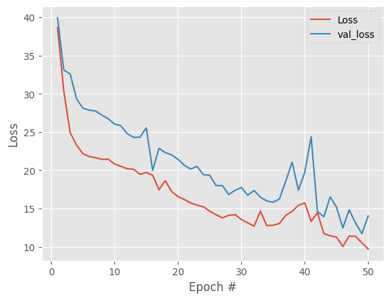
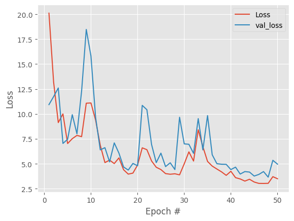
check how validation behaves over time (epochs)
1import matplotlib.pyplot as plt
2plt.style.use("ggplot")
3plt.plot(np.arange(1, epochs + 1), H.history["loss"], label="Loss")
4plt.plot(np.arange(1, epochs + 1), H.history["val_loss"], label="val_loss")
5plt.xlabel("Epoch #")
6plt.ylabel("Loss")
7plt.legend()
8plt.show()
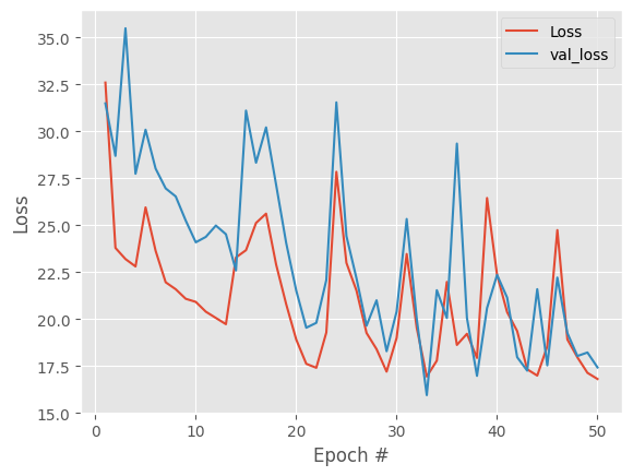
We see both training and validation loss are extremely noisy, with no clear improvement trend, and after ~15-20 epochs, improvements are just random fluctuations, not learning.
In these cases, it is useful to add regularization and decrease learning rate.
Regularization refers to a set of techniques used to reduce overfitting by discouraging overly complex models, typically by adding a penalty to the training objective that constrains model parameters. This encourages the model to learn more generalizable patterns rather than memorizing noise in the data.
L2 regularization (also known as weight decay) adds a penalty proportional to the sum of the squared model weights to the loss function, pushing weights toward smaller values without forcing them to zero. This helps stabilize training and promotes smoother, less sensitive models.
 1from tensorflow.keras import regularizers
 2
 3def create_l2_autoencoder(neurons, input_shape, l2=1e-5):
 4    input_layer = Input(shape=(input_shape,))
 5
 6    # Encoder layers
 7    encoder_output = input_layer
 8    for i in range(len(neurons)-1, 0, -1):
 9        encoder_output = Dense(neurons[i], activation='elu',
10            kernel_regularizer=regularizers.l2(l2))(encoder_output)
11
12    # Hidden layer with a name
13    hidden_layer = Dense(neurons[0], activation='linear', name='hidden_layer',
14            kernel_regularizer=regularizers.l2(l2))(encoder_output)
15
16    # Decoder layers
17    decoder_output = hidden_layer
18    for i in range(1, len(neurons)):
19        decoder_output = Dense(neurons[i], activation='elu',
20            kernel_regularizer=regularizers.l2(l2))(decoder_output)
21
22    # Output layer
23    output_layer = Dense(input_shape, activation='linear')(decoder_output)
24
25    autoencoder = Model(inputs=input_layer, outputs=output_layer)
26    return autoencoder
re-initialize the model before running .fit() again to avoid keep training the same model
 1autoencoder = create_l2_autoencoder(
 2    neurons,
 3    train_data.shape[1],
 4    l2=1e-5
 5)
 6
 7optimizer = tf.keras.optimizers.Adam(learning_rate=1e-3)
 8autoencoder.compile(
 9    optimizer=optimizer,
10    loss='mean_squared_error'
11)
12
13H = autoencoder.fit(
14    train_data,
15    train_data,
16    validation_data=(test_data, test_data),
17    batch_size=32,
18    epochs=epochs,
19    verbose=1
20)
  1Epoch 1/50
  293/93 [==============================] - 5s 16ms/step - loss: 26.6187 - val_loss: 27.4128
  3Epoch 2/50
  493/93 [==============================] - 1s 16ms/step - loss: 20.0764 - val_loss: 22.8442
  5Epoch 3/50
  693/93 [==============================] - 2s 17ms/step - loss: 16.3306 - val_loss: 19.9515
  7Epoch 4/50
  893/93 [==============================] - 1s 14ms/step - loss: 13.2374 - val_loss: 17.0505
  9Epoch 5/50
 1093/93 [==============================] - 2s 17ms/step - loss: 11.6092 - val_loss: 10.3541
 11Epoch 6/50
 1293/93 [==============================] - 2s 18ms/step - loss: 12.8784 - val_loss: 18.2110
 13Epoch 7/50
 1493/93 [==============================] - 1s 16ms/step - loss: 11.9601 - val_loss: 11.6533
 15Epoch 8/50
 1693/93 [==============================] - 1s 15ms/step - loss: 10.6742 - val_loss: 10.2509
 17Epoch 9/50
 1893/93 [==============================] - 1s 13ms/step - loss: 11.4126 - val_loss: 19.5551
 19Epoch 10/50
 2093/93 [==============================] - 2s 16ms/step - loss: 11.7762 - val_loss: 12.6366
 21Epoch 11/50
 2293/93 [==============================] - 1s 12ms/step - loss: 10.6223 - val_loss: 11.3330
 23Epoch 12/50
 2493/93 [==============================] - 2s 17ms/step - loss: 9.4480 - val_loss: 8.9790
 25Epoch 13/50
 2693/93 [==============================] - 2s 18ms/step - loss: 9.4324 - val_loss: 11.6798
 27Epoch 14/50
 2893/93 [==============================] - 2s 17ms/step - loss: 9.1592 - val_loss: 9.1531
 29Epoch 15/50
 3093/93 [==============================] - 1s 14ms/step - loss: 8.1193 - val_loss: 7.4658
 31Epoch 16/50
 3293/93 [==============================] - 1s 12ms/step - loss: 8.5194 - val_loss: 9.5459
 33Epoch 17/50
 3493/93 [==============================] - 2s 19ms/step - loss: 8.9682 - val_loss: 10.1431
 35Epoch 18/50
 3693/93 [==============================] - 2s 18ms/step - loss: 8.8097 - val_loss: 9.3160
 37Epoch 19/50
 3893/93 [==============================] - 1s 12ms/step - loss: 9.3907 - val_loss: 9.4668
 39Epoch 20/50
 4093/93 [==============================] - 2s 18ms/step - loss: 9.1025 - val_loss: 8.1897
 41Epoch 21/50
 4293/93 [==============================] - 1s 13ms/step - loss: 8.5533 - val_loss: 8.7505
 43Epoch 22/50
 4493/93 [==============================] - 2s 19ms/step - loss: 7.8477 - val_loss: 9.3622
 45Epoch 23/50
 4693/93 [==============================] - 1s 14ms/step - loss: 7.1622 - val_loss: 7.6489
 47Epoch 24/50
 4893/93 [==============================] - 2s 17ms/step - loss: 8.5040 - val_loss: 7.6554
 49Epoch 25/50
 5093/93 [==============================] - 2s 16ms/step - loss: 7.7141 - val_loss: 6.8418
 51Epoch 26/50
 5293/93 [==============================] - 1s 9ms/step - loss: 7.2177 - val_loss: 9.9998
 53Epoch 27/50
 5493/93 [==============================] - 1s 14ms/step - loss: 9.1925 - val_loss: 10.6097
 55Epoch 28/50
 5693/93 [==============================] - 1s 11ms/step - loss: 9.3420 - val_loss: 7.8157
 57Epoch 29/50
 5893/93 [==============================] - 1s 12ms/step - loss: 7.7143 - val_loss: 6.8660
 59Epoch 30/50
 6093/93 [==============================] - 2s 17ms/step - loss: 8.0236 - val_loss: 7.9869
 61Epoch 31/50
 6293/93 [==============================] - 2s 17ms/step - loss: 7.6223 - val_loss: 7.6642
 63Epoch 32/50
 6493/93 [==============================] - 1s 7ms/step - loss: 7.7311 - val_loss: 8.0535
 65Epoch 33/50
 6693/93 [==============================] - 1s 6ms/step - loss: 7.9626 - val_loss: 12.3125
 67Epoch 34/50
 6893/93 [==============================] - 1s 10ms/step - loss: 9.5091 - val_loss: 8.1515
 69Epoch 35/50
 7093/93 [==============================] - 1s 11ms/step - loss: 12.8089 - val_loss: 8.4810
 71Epoch 36/50
 7293/93 [==============================] - 1s 15ms/step - loss: 10.1668 - val_loss: 11.3264
 73Epoch 37/50
 7493/93 [==============================] - 1s 7ms/step - loss: 11.6888 - val_loss: 21.4890
 75Epoch 38/50
 7693/93 [==============================] - 1s 9ms/step - loss: 12.3693 - val_loss: 11.9961
 77Epoch 39/50
 7893/93 [==============================] - 1s 11ms/step - loss: 10.7251 - val_loss: 10.1258
 79Epoch 40/50
 8093/93 [==============================] - 1s 9ms/step - loss: 8.8597 - val_loss: 7.9398
 81Epoch 41/50
 8293/93 [==============================] - 1s 12ms/step - loss: 8.0705 - val_loss: 7.6555
 83Epoch 42/50
 8493/93 [==============================] - 1s 13ms/step - loss: 7.3514 - val_loss: 7.2101
 85Epoch 43/50
 8693/93 [==============================] - 1s 16ms/step - loss: 6.8367 - val_loss: 7.4991
 87Epoch 44/50
 8893/93 [==============================] - 2s 17ms/step - loss: 7.1375 - val_loss: 7.3583
 89Epoch 45/50
 9093/93 [==============================] - 1s 12ms/step - loss: 7.2660 - val_loss: 8.2415
 91Epoch 46/50
 9293/93 [==============================] - 2s 18ms/step - loss: 7.7464 - val_loss: 7.1394
 93Epoch 47/50
 9493/93 [==============================] - 1s 15ms/step - loss: 7.0515 - val_loss: 6.6802
 95Epoch 48/50
 9693/93 [==============================] - 2s 16ms/step - loss: 6.8640 - val_loss: 7.2763
 97Epoch 49/50
 9893/93 [==============================] - 1s 13ms/step - loss: 6.8215 - val_loss: 6.4784
 99Epoch 50/50
10093/93 [==============================] - 1s 15ms/step - loss: 7.0084 - val_loss: 7.1828
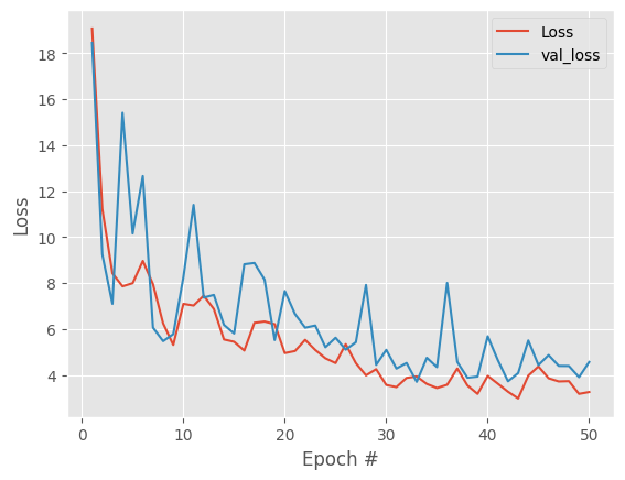
and plot the losses
1plt.style.use("ggplot")
2N = len(H.history["loss"])
3plt.plot(np.arange(1, N + 1), H.history["loss"], label="Loss")
4plt.plot(np.arange(1, N + 1), H.history["val_loss"], label="val_loss")
5plt.xlabel("Epoch #")
6plt.ylabel("Loss")
7plt.legend()
8plt.show()
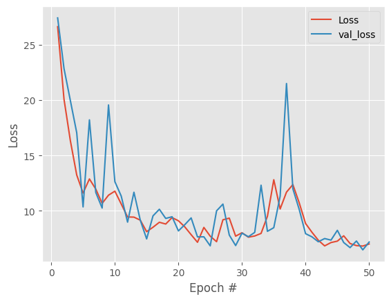
there is a clear improvement but we still have some large spikes and improvements after ~20 epochs are basically noise. With our data, one possible cause is data noise / dropout so we will input noise and repeat the whole process.
 1from tensorflow.keras.layers import GaussianNoise
 2
 3def create_l2_noise_autoencoder(neurons, input_shape, l2=1e-5, noise_std=0.1):
 4    input_layer = Input(shape=(input_shape,))
 5    x = GaussianNoise(noise_std)(input_layer)
 6
 7    # Encoder layers
 8    encoder_output = x
 9    for i in range(len(neurons)-1, 0, -1):
10        encoder_output = Dense(neurons[i], activation='elu',
11            kernel_regularizer=regularizers.l2(l2))(encoder_output)
12
13    # Hidden layer with a name
14    hidden_layer = Dense(neurons[0], activation='linear', name='hidden_layer',
15            kernel_regularizer=regularizers.l2(l2))(encoder_output)
16
17    # Decoder layers
18    decoder_output = hidden_layer
19    for i in range(1, len(neurons)):
20        decoder_output = Dense(neurons[i], activation='elu',
21            kernel_regularizer=regularizers.l2(l2))(decoder_output)
22
23    # Output layer
24    output_layer = Dense(input_shape, activation='linear')(decoder_output)
25
26    autoencoder = Model(inputs=input_layer, outputs=output_layer)
27    return autoencoder
 1autoencoder = create_l2_noise_autoencoder(
 2    neurons,
 3    train_data.shape[1],
 4    l2=1e-5,
 5    noise_std=0.1
 6)
 7
 8optimizer = tf.keras.optimizers.Adam(learning_rate=1e-3)
 9autoencoder.compile(
10    optimizer=optimizer,
11    loss='mean_squared_error'
12)
13
14H = autoencoder.fit(
15    train_data,
16    train_data,
17    validation_data=(test_data, test_data),
18    batch_size=32,
19    epochs=epochs,
20    verbose=1
21)
  1Epoch 1/50
  293/93 [==============================] - 4s 11ms/step - loss: 31.7372 - val_loss: 30.9056
  3Epoch 2/50
  493/93 [==============================] - 1s 16ms/step - loss: 24.1195 - val_loss: 30.1557
  5Epoch 3/50
  693/93 [==============================] - 1s 12ms/step - loss: 22.7737 - val_loss: 28.8883
  7Epoch 4/50
  893/93 [==============================] - 1s 12ms/step - loss: 22.4682 - val_loss: 28.5310
  9Epoch 5/50
 1093/93 [==============================] - 1s 13ms/step - loss: 22.3388 - val_loss: 27.8151
 11Epoch 6/50
 1293/93 [==============================] - 1s 16ms/step - loss: 22.3382 - val_loss: 31.0888
 13Epoch 7/50
 1493/93 [==============================] - 1s 15ms/step - loss: 22.1720 - val_loss: 27.5932
 15Epoch 8/50
 1693/93 [==============================] - 1s 13ms/step - loss: 21.6034 - val_loss: 27.3644
 17Epoch 9/50
 1893/93 [==============================] - 1s 9ms/step - loss: 22.4259 - val_loss: 31.4528
 19Epoch 10/50
 2093/93 [==============================] - 1s 15ms/step - loss: 22.8885 - val_loss: 28.0888
 21Epoch 11/50
 2293/93 [==============================] - 1s 12ms/step - loss: 21.8866 - val_loss: 26.8629
 23Epoch 12/50
 2493/93 [==============================] - 1s 15ms/step - loss: 21.5496 - val_loss: 27.7277
 25Epoch 13/50
 2693/93 [==============================] - 1s 14ms/step - loss: 21.3155 - val_loss: 26.2743
 27Epoch 14/50
 2893/93 [==============================] - 1s 13ms/step - loss: 22.5453 - val_loss: 25.7421
 29Epoch 15/50
 3093/93 [==============================] - 2s 17ms/step - loss: 20.7408 - val_loss: 25.2304
 31Epoch 16/50
 3293/93 [==============================] - 1s 12ms/step - loss: 20.3711 - val_loss: 25.2569
 33Epoch 17/50
 3493/93 [==============================] - 1s 16ms/step - loss: 19.8909 - val_loss: 23.9351
 35Epoch 18/50
 3693/93 [==============================] - 1s 14ms/step - loss: 19.7199 - val_loss: 23.9300
 37Epoch 19/50
 3893/93 [==============================] - 1s 14ms/step - loss: 19.2602 - val_loss: 23.2457
 39Epoch 20/50
 4093/93 [==============================] - 1s 15ms/step - loss: 18.9191 - val_loss: 22.8827
 41Epoch 21/50
 4293/93 [==============================] - 1s 14ms/step - loss: 18.5888 - val_loss: 23.1114
 43Epoch 22/50
 4493/93 [==============================] - 1s 16ms/step - loss: 18.4964 - val_loss: 22.9688
 45Epoch 23/50
 4693/93 [==============================] - 1s 11ms/step - loss: 18.6124 - val_loss: 22.2674
 47Epoch 24/50
 4893/93 [==============================] - 2s 17ms/step - loss: 17.7730 - val_loss: 23.0081
 49Epoch 25/50
 5093/93 [==============================] - 1s 9ms/step - loss: 18.0176 - val_loss: 21.7493
 51Epoch 26/50
 5293/93 [==============================] - 1s 9ms/step - loss: 17.4766 - val_loss: 20.5798
 53Epoch 27/50
 5493/93 [==============================] - 1s 15ms/step - loss: 17.2889 - val_loss: 20.2625
 55Epoch 28/50
 5693/93 [==============================] - 1s 16ms/step - loss: 17.4654 - val_loss: 23.4170
 57Epoch 29/50
 5893/93 [==============================] - 1s 10ms/step - loss: 16.9935 - val_loss: 20.6892
 59Epoch 30/50
 6093/93 [==============================] - 1s 13ms/step - loss: 28.9395 - val_loss: 68.7133
 61Epoch 31/50
 6293/93 [==============================] - 1s 15ms/step - loss: 27.4823 - val_loss: 27.9025
 63Epoch 32/50
 6493/93 [==============================] - 1s 14ms/step - loss: 21.1761 - val_loss: 24.7234
 65Epoch 33/50
 6693/93 [==============================] - 2s 16ms/step - loss: 19.8319 - val_loss: 24.1620
 67Epoch 34/50
 6893/93 [==============================] - 1s 14ms/step - loss: 19.3813 - val_loss: 23.4190
 69Epoch 35/50
 7093/93 [==============================] - 1s 14ms/step - loss: 18.8075 - val_loss: 22.6499
 71Epoch 36/50
 7293/93 [==============================] - 1s 12ms/step - loss: 19.0569 - val_loss: 22.2925
 73Epoch 37/50
 7493/93 [==============================] - 1s 10ms/step - loss: 18.8629 - val_loss: 22.6711
 75Epoch 38/50
 7693/93 [==============================] - 1s 15ms/step - loss: 16.1751 - val_loss: 16.3366
 77Epoch 39/50
 7893/93 [==============================] - 2s 18ms/step - loss: 14.4210 - val_loss: 15.0888
 79Epoch 40/50
 8093/93 [==============================] - 2s 16ms/step - loss: 13.0786 - val_loss: 13.6408
 81Epoch 41/50
 8293/93 [==============================] - 2s 17ms/step - loss: 12.8257 - val_loss: 14.2111
 83Epoch 42/50
 8493/93 [==============================] - 1s 15ms/step - loss: 12.2966 - val_loss: 13.4075
 85Epoch 43/50
 8693/93 [==============================] - 1s 11ms/step - loss: 11.4765 - val_loss: 11.9199
 87Epoch 44/50
 8893/93 [==============================] - 1s 14ms/step - loss: 12.7848 - val_loss: 14.4697
 89Epoch 45/50
 9093/93 [==============================] - 1s 10ms/step - loss: 18.1168 - val_loss: 17.5223
 91Epoch 46/50
 9293/93 [==============================] - 1s 14ms/step - loss: 14.1584 - val_loss: 15.3487
 93Epoch 47/50
 9493/93 [==============================] - 1s 14ms/step - loss: 12.4028 - val_loss: 13.6837
 95Epoch 48/50
 9693/93 [==============================] - 1s 16ms/step - loss: 11.8782 - val_loss: 12.1098
 97Epoch 49/50
 9893/93 [==============================] - 2s 16ms/step - loss: 10.6474 - val_loss: 11.5075
 99Epoch 50/50
10093/93 [==============================] - 1s 11ms/step - loss: 10.1763 - val_loss: 11.3282
1plt.style.use("ggplot")
2N = len(H.history["loss"])
3plt.plot(np.arange(1, N + 1), H.history["loss"], label="Loss")
4plt.plot(np.arange(1, N + 1), H.history["val_loss"], label="val_loss")
5plt.xlabel("Epoch #")
6plt.ylabel("Loss")
7plt.legend()
8plt.show()
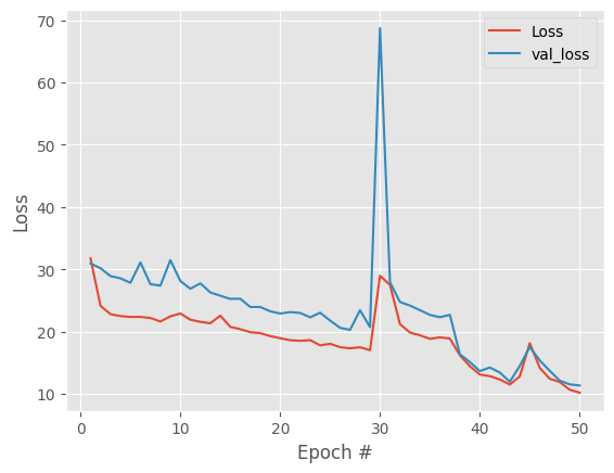
Good result, overall downward trend in both losses and track each other. Model is not overfitting. To remove the spikes in losses and get more stable embeddings lets try decreasing the learning rate.
 1autoencoder = create_l2_noise_autoencoder(
 2    neurons,
 3    train_data.shape[1],
 4    l2=1e-5,
 5    noise_std=0.1
 6)
 7
 8optimizer = tf.keras.optimizers.Adam(learning_rate=3e-4)
 9autoencoder.compile(
10    optimizer=optimizer,
11    loss='mean_squared_error'
12)
13
14H = autoencoder.fit(
15    train_data,
16    train_data,
17    validation_data=(test_data, test_data),
18    batch_size=32,
19    epochs=epochs,
20    verbose=1
21)
  1Epoch 1/50
  293/93 [==============================] - 5s 15ms/step - loss: 38.6527 - val_loss: 39.9125
  3Epoch 2/50
  493/93 [==============================] - 1s 13ms/step - loss: 30.2958 - val_loss: 33.0952
  5Epoch 3/50
  693/93 [==============================] - 2s 18ms/step - loss: 24.9085 - val_loss: 32.5780
  7Epoch 4/50
  893/93 [==============================] - 1s 13ms/step - loss: 23.2918 - val_loss: 29.3479
  9Epoch 5/50
 1093/93 [==============================] - 1s 15ms/step - loss: 22.1767 - val_loss: 28.1120
 11Epoch 6/50
 1293/93 [==============================] - 1s 16ms/step - loss: 21.7849 - val_loss: 27.8594
 13Epoch 7/50
 1493/93 [==============================] - 1s 12ms/step - loss: 21.6366 - val_loss: 27.7357
 15Epoch 8/50
 1693/93 [==============================] - 1s 15ms/step - loss: 21.4320 - val_loss: 27.2052
 17Epoch 9/50
 1893/93 [==============================] - 1s 14ms/step - loss: 21.4469 - val_loss: 26.7283
 19Epoch 10/50
 2093/93 [==============================] - 2s 16ms/step - loss: 20.8234 - val_loss: 26.0348
 21Epoch 11/50
 2293/93 [==============================] - 2s 17ms/step - loss: 20.5192 - val_loss: 25.8189
 23Epoch 12/50
 2493/93 [==============================] - 1s 12ms/step - loss: 20.2020 - val_loss: 24.7882
 25Epoch 13/50
 2693/93 [==============================] - 1s 12ms/step - loss: 20.1402 - val_loss: 24.2947
 27Epoch 14/50
 2893/93 [==============================] - 1s 14ms/step - loss: 19.4716 - val_loss: 24.3214
 29Epoch 15/50
 3093/93 [==============================] - 2s 18ms/step - loss: 19.7134 - val_loss: 25.5420
 31Epoch 16/50
 3293/93 [==============================] - 1s 16ms/step - loss: 19.3621 - val_loss: 19.9822
 33Epoch 17/50
 3493/93 [==============================] - 1s 13ms/step - loss: 17.4665 - val_loss: 22.8801
 35Epoch 18/50
 3693/93 [==============================] - 1s 13ms/step - loss: 18.6423 - val_loss: 22.3084
 37Epoch 19/50
 3893/93 [==============================] - 1s 15ms/step - loss: 17.2165 - val_loss: 22.0067
 39Epoch 20/50
 4093/93 [==============================] - 1s 10ms/step - loss: 16.5752 - val_loss: 21.4383
 41Epoch 21/50
 4293/93 [==============================] - 1s 12ms/step - loss: 16.1724 - val_loss: 20.6535
 43Epoch 22/50
 4493/93 [==============================] - 1s 12ms/step - loss: 15.7307 - val_loss: 20.1583
 45Epoch 23/50
 4693/93 [==============================] - 1s 15ms/step - loss: 15.4491 - val_loss: 20.5153
 47Epoch 24/50
 4893/93 [==============================] - 1s 8ms/step - loss: 15.2299 - val_loss: 19.4298
 49Epoch 25/50
 5093/93 [==============================] - 1s 14ms/step - loss: 14.6663 - val_loss: 19.3464
 51Epoch 26/50
 5293/93 [==============================] - 1s 12ms/step - loss: 14.2106 - val_loss: 18.0098
 53Epoch 27/50
 5493/93 [==============================] - 1s 15ms/step - loss: 13.7767 - val_loss: 18.0012
 55Epoch 28/50
 5693/93 [==============================] - 1s 13ms/step - loss: 14.1194 - val_loss: 16.8258
 57Epoch 29/50
 5893/93 [==============================] - 1s 15ms/step - loss: 14.2060 - val_loss: 17.3795
 59Epoch 30/50
 6093/93 [==============================] - 1s 14ms/step - loss: 13.5694 - val_loss: 17.7462
 61Epoch 31/50
 6293/93 [==============================] - 2s 16ms/step - loss: 13.1289 - val_loss: 16.7373
 63Epoch 32/50
 6493/93 [==============================] - 1s 9ms/step - loss: 12.7070 - val_loss: 17.3542
 65Epoch 33/50
 6693/93 [==============================] - 1s 15ms/step - loss: 14.6508 - val_loss: 16.4855
 67Epoch 34/50
 6893/93 [==============================] - 1s 13ms/step - loss: 12.7817 - val_loss: 15.9853
 69Epoch 35/50
 7093/93 [==============================] - 1s 16ms/step - loss: 12.8153 - val_loss: 15.8276
 71Epoch 36/50
 7293/93 [==============================] - 1s 15ms/step - loss: 13.0446 - val_loss: 16.2531
 73Epoch 37/50
 7493/93 [==============================] - 1s 16ms/step - loss: 14.1267 - val_loss: 18.5714
 75Epoch 38/50
 7693/93 [==============================] - 1s 14ms/step - loss: 14.6227 - val_loss: 21.0582
 77Epoch 39/50
 7893/93 [==============================] - 1s 14ms/step - loss: 15.4332 - val_loss: 17.4142
 79Epoch 40/50
 8093/93 [==============================] - 1s 12ms/step - loss: 15.7435 - val_loss: 19.7408
 81Epoch 41/50
 8293/93 [==============================] - 1s 15ms/step - loss: 13.3249 - val_loss: 24.3964
 83Epoch 42/50
 8493/93 [==============================] - 1s 12ms/step - loss: 14.4557 - val_loss: 14.6062
 85Epoch 43/50
 8693/93 [==============================] - 1s 14ms/step - loss: 11.7363 - val_loss: 13.9266
 87Epoch 44/50
 8893/93 [==============================] - 1s 13ms/step - loss: 11.4413 - val_loss: 16.5276
 89Epoch 45/50
 9093/93 [==============================] - 1s 13ms/step - loss: 11.2720 - val_loss: 15.1880
 91Epoch 46/50
 9293/93 [==============================] - 1s 14ms/step - loss: 10.0483 - val_loss: 12.4647
 93Epoch 47/50
 9493/93 [==============================] - 1s 16ms/step - loss: 11.4013 - val_loss: 14.8307
 95Epoch 48/50
 9693/93 [==============================] - 1s 11ms/step - loss: 11.3730 - val_loss: 13.1132
 97Epoch 49/50
 9893/93 [==============================] - 1s 12ms/step - loss: 10.5250 - val_loss: 11.7176
 99Epoch 50/50
10093/93 [==============================] - 1s 15ms/step - loss: 9.7135 - val_loss: 14.0300
1plt.style.use("ggplot")
2N = len(H.history["loss"])
3plt.plot(np.arange(1, N + 1), H.history["loss"], label="Loss")
4plt.plot(np.arange(1, N + 1), H.history["val_loss"], label="val_loss")
5plt.xlabel("Epoch #")
6plt.ylabel("Loss")
7plt.legend()
8plt.show()
at this point we can extract the hidden layer or bottleneck to use it as dimensional reduction coordinates in our pancreatic cells sce object.
1hidden_layer_model = Model(inputs=autoencoder.input, outputs=autoencoder.get_layer('hidden_layer').output)
2hidden_layer_values = hidden_layer_model.predict(input_data)
1116/116 [==============================] - 0s 1ms/step
1print("Shape of hidden layer values:", hidden_layer_values.shape)
1Shape of hidden layer values: (3696, 2)
and save it to disk to open it outside docker
1hidden_layer_array = np.array(hidden_layer_values)
2hidden_layer_df = pd.DataFrame(hidden_layer_array, columns=[f'Autoencoder_{i}' for i in range(hidden_layer_array.shape[1])])
3csv_output_path = 'hidden_layer.docker.1024.4.hidden2.earlystop.fixPreprocessing.csv'
4hidden_layer_df.to_csv(csv_output_path, index=False)
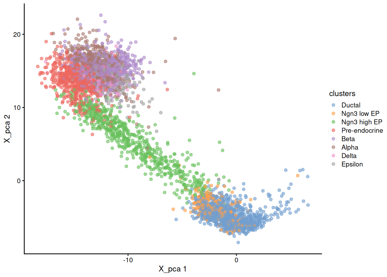
now let's get back to R (or python) outside docker and plot the original PCA
1library(scater)
2plotReducedDim( sce, dimred = 'X_pca', colour_by='clusters' )
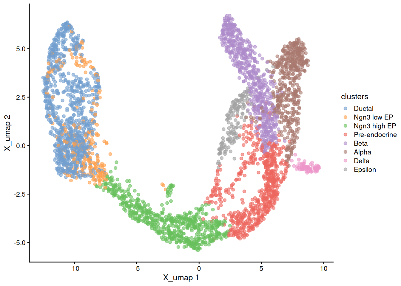
and the original UMAP
1plotReducedDim( sce, dimred = 'X_umap', colour_by='clusters' )
now we read the autoencoder bottleneck data and add it to the SCE reducedDim slot.
1autoencoder.df <- read.csv( 'hidden_layer.docker.1024.4.hidden2.earlystop.fixPreprocessing.csv' )
2rownames(autoencoder.df) <- colnames(sce)
3reducedDim( sce, 'AE' ) <- autoencoder.df
now plot the results
1plotReducedDim( sce, dimred = 'AE', colour_by='clusters' )
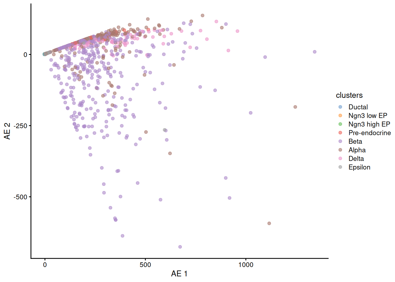
It seems our basic AE is not good enough to be used directly to plot the cells.
Next we will try to use the same autoencoder approach but defining a 50 neuron bottleneck that we will use later as the basis to the tSNE and UMAP representations as we normally do with PCA.
Open a new jupyter notebook inside the docker and do the same until defining the number of neurons per layer
1neurons = [50] + [2**x for x in range(6,11)]
2neurons
1[50, 64, 128, 256, 512, 1024]
learning rate and the number of epochs
1custom_learning_rate = 0.001
2epochs = 50
autoencoder function
 1def create_autoencoder(neurons, input_shape):
 2    input_layer = Input(shape=(input_shape,))
 3
 4    # Encoder layers
 5    encoder_output = input_layer
 6    for i in range(len(neurons)-1, 0, -1):
 7        encoder_output = Dense(neurons[i], activation='elu')(encoder_output)
 8
 9    # Hidden layer with a name
10    hidden_layer = Dense(neurons[0], activation='linear', name='hidden_layer')(encoder_output)
11
12    # Decoder layers
13    decoder_output = hidden_layer
14    for i in range(1, len(neurons)):
15        decoder_output = Dense(neurons[i], activation='elu')(decoder_output)
16
17    # Output layer
18    output_layer = Dense(input_shape, activation='linear')(decoder_output)
19    # output_layer = Dense(input_shape, activation='sigmoid')(decoder_output) # changed because input goes from -1 to 1
20
21    autoencoder = Model(inputs=input_layer, outputs=output_layer)
22    return autoencoder
autoencoder set up
1autoencoder = create_autoencoder(neurons, train_data.shape[1])
 12025-12-17 17:28:28.376131: I external/local_xla/xla/stream_executor/cuda/cuda_executor.cc:901] successful NUMA node read from SysFS had negative value (-1), but there must be at least one NUMA node, so returning NUMA node zero. See more at https://github.com/torvalds/linux/blob/v6.0/Documentation/ABI/testing/sysfs-bus-pci#L344-L355
 22025-12-17 17:28:28.437362: I external/local_xla/xla/stream_executor/cuda/cuda_executor.cc:901] successful NUMA node read from SysFS had negative value (-1), but there must be at least one NUMA node, so returning NUMA node zero. See more at https://github.com/torvalds/linux/blob/v6.0/Documentation/ABI/testing/sysfs-bus-pci#L344-L355
 32025-12-17 17:28:28.440064: I external/local_xla/xla/stream_executor/cuda/cuda_executor.cc:901] successful NUMA node read from SysFS had negative value (-1), but there must be at least one NUMA node, so returning NUMA node zero. See more at https://github.com/torvalds/linux/blob/v6.0/Documentation/ABI/testing/sysfs-bus-pci#L344-L355
 42025-12-17 17:28:28.443025: I external/local_xla/xla/stream_executor/cuda/cuda_executor.cc:901] successful NUMA node read from SysFS had negative value (-1), but there must be at least one NUMA node, so returning NUMA node zero. See more at https://github.com/torvalds/linux/blob/v6.0/Documentation/ABI/testing/sysfs-bus-pci#L344-L355
 52025-12-17 17:28:28.445118: I external/local_xla/xla/stream_executor/cuda/cuda_executor.cc:901] successful NUMA node read from SysFS had negative value (-1), but there must be at least one NUMA node, so returning NUMA node zero. See more at https://github.com/torvalds/linux/blob/v6.0/Documentation/ABI/testing/sysfs-bus-pci#L344-L355
 62025-12-17 17:28:28.450453: I external/local_xla/xla/stream_executor/cuda/cuda_executor.cc:901] successful NUMA node read from SysFS had negative value (-1), but there must be at least one NUMA node, so returning NUMA node zero. See more at https://github.com/torvalds/linux/blob/v6.0/Documentation/ABI/testing/sysfs-bus-pci#L344-L355
 72025-12-17 17:28:28.598267: I external/local_xla/xla/stream_executor/cuda/cuda_executor.cc:901] successful NUMA node read from SysFS had negative value (-1), but there must be at least one NUMA node, so returning NUMA node zero. See more at https://github.com/torvalds/linux/blob/v6.0/Documentation/ABI/testing/sysfs-bus-pci#L344-L355
 82025-12-17 17:28:28.599087: I external/local_xla/xla/stream_executor/cuda/cuda_executor.cc:901] successful NUMA node read from SysFS had negative value (-1), but there must be at least one NUMA node, so returning NUMA node zero. See more at https://github.com/torvalds/linux/blob/v6.0/Documentation/ABI/testing/sysfs-bus-pci#L344-L355
 92025-12-17 17:28:28.599764: I external/local_xla/xla/stream_executor/cuda/cuda_executor.cc:901] successful NUMA node read from SysFS had negative value (-1), but there must be at least one NUMA node, so returning NUMA node zero. See more at https://github.com/torvalds/linux/blob/v6.0/Documentation/ABI/testing/sysfs-bus-pci#L344-L355
102025-12-17 17:28:28.600633: I tensorflow/core/common_runtime/gpu/gpu_device.cc:1929] Created device /job:localhost/replica:0/task:0/device:GPU:0 with 6002 MB memory:  -> device: 0, name: NVIDIA GeForce RTX 2070 SUPER, pci bus id: 0000:01:00.0, compute capability: 7.5
optimizer and compilation
1optimizer = tf.keras.optimizers.Adam(learning_rate=custom_learning_rate)
2autoencoder.compile(optimizer=optimizer, loss='mean_squared_error')
model summary
1autoencoder.summary()
 1Model: "model"
 2_________________________________________________________________
 3 Layer (type)                Output Shape              Param #
 4=================================================================
 5 input_1 (InputLayer)        [(None, 2000)]            0
 6
 7 dense (Dense)               (None, 1024)              2049024
 8
 9 dense_1 (Dense)             (None, 512)               524800
10
11 dense_2 (Dense)             (None, 256)               131328
12
13 dense_3 (Dense)             (None, 128)               32896
14
15 dense_4 (Dense)             (None, 64)                8256
16
17 hidden_layer (Dense)        (None, 50)                3250
18
19 dense_5 (Dense)             (None, 64)                3264
20
21 dense_6 (Dense)             (None, 128)               8320
22
23 dense_7 (Dense)             (None, 256)               33024
24
25 dense_8 (Dense)             (None, 512)               131584
26
27 dense_9 (Dense)             (None, 1024)              525312
28
29 dense_10 (Dense)            (None, 2000)              2050000
30
31=================================================================
32Total params: 5501058 (20.98 MB)
33Trainable params: 5501058 (20.98 MB)
34Non-trainable params: 0 (0.00 Byte)
35_________________________________________________________________
training
1H = autoencoder.fit(x = train_data, y = train_data,
2                    validation_data=(test_data, test_data),
3                    batch_size = 32, epochs = epochs, verbose = 1)
  1Epoch 1/50
  2
  3
  42025-12-17 17:29:12.731974: I external/local_xla/xla/service/service.cc:168] XLA service 0x76a550615c30 initialized for platform CUDA (this does not guarantee that XLA will be used). Devices:
  52025-12-17 17:29:12.731994: I external/local_xla/xla/service/service.cc:176]   StreamExecutor device (0): NVIDIA GeForce RTX 2070 SUPER, Compute Capability 7.5
  62025-12-17 17:29:12.741006: I tensorflow/compiler/mlir/tensorflow/utils/dump_mlir_util.cc:269] disabling MLIR crash reproducer, set env var `MLIR_CRASH_REPRODUCER_DIRECTORY` to enable.
  72025-12-17 17:29:12.761897: I external/local_xla/xla/stream_executor/cuda/cuda_dnn.cc:454] Loaded cuDNN version 8906
  8WARNING: All log messages before absl::InitializeLog() is called are written to STDERR
  9I0000 00:00:1765992552.816020     271 device_compiler.h:186] Compiled cluster using XLA!  This line is logged at most once for the lifetime of the process.
 10
 11
 1293/93 [==============================] - 4s 11ms/step - loss: 20.1129 - val_loss: 10.9373
 13Epoch 2/50
 1493/93 [==============================] - 1s 13ms/step - loss: 13.1907 - val_loss: 11.7414
 15Epoch 3/50
 1693/93 [==============================] - 1s 14ms/step - loss: 9.1359 - val_loss: 12.6089
 17Epoch 4/50
 1893/93 [==============================] - 1s 12ms/step - loss: 10.0069 - val_loss: 7.0463
 19Epoch 5/50
 2093/93 [==============================] - 1s 13ms/step - loss: 7.0336 - val_loss: 7.4595
 21Epoch 6/50
 2293/93 [==============================] - 1s 9ms/step - loss: 7.5198 - val_loss: 9.9332
 23Epoch 7/50
 2493/93 [==============================] - 1s 8ms/step - loss: 7.8503 - val_loss: 8.0087
 25Epoch 8/50
 2693/93 [==============================] - 1s 12ms/step - loss: 7.7250 - val_loss: 12.2940
 27Epoch 9/50
 2893/93 [==============================] - 1s 11ms/step - loss: 11.0793 - val_loss: 18.4790
 29Epoch 10/50
 3093/93 [==============================] - 1s 9ms/step - loss: 11.1037 - val_loss: 15.8162
 31Epoch 11/50
 3293/93 [==============================] - 1s 12ms/step - loss: 9.3877 - val_loss: 9.6597
 33Epoch 12/50
 3493/93 [==============================] - 1s 12ms/step - loss: 6.8708 - val_loss: 6.3998
 35Epoch 13/50
 3693/93 [==============================] - 1s 12ms/step - loss: 5.1222 - val_loss: 6.6202
 37Epoch 14/50
 3893/93 [==============================] - 1s 12ms/step - loss: 5.3738 - val_loss: 5.1922
 39Epoch 15/50
 4093/93 [==============================] - 1s 8ms/step - loss: 5.0246 - val_loss: 7.0998
 41Epoch 16/50
 4293/93 [==============================] - 1s 11ms/step - loss: 5.5951 - val_loss: 6.0730
 43Epoch 17/50
 4493/93 [==============================] - 1s 9ms/step - loss: 4.4057 - val_loss: 4.6819
 45Epoch 18/50
 4693/93 [==============================] - 1s 9ms/step - loss: 3.9670 - val_loss: 4.3718
 47Epoch 19/50
 4893/93 [==============================] - 1s 12ms/step - loss: 4.0684 - val_loss: 5.0374
 49Epoch 20/50
 5093/93 [==============================] - 1s 7ms/step - loss: 4.8767 - val_loss: 4.8057
 51Epoch 21/50
 5293/93 [==============================] - 1s 13ms/step - loss: 6.6046 - val_loss: 10.8622
 53Epoch 22/50
 5493/93 [==============================] - 1s 13ms/step - loss: 6.4166 - val_loss: 10.4268
 55Epoch 23/50
 5693/93 [==============================] - 1s 10ms/step - loss: 5.2859 - val_loss: 6.9333
 57Epoch 24/50
 5893/93 [==============================] - 1s 13ms/step - loss: 4.6556 - val_loss: 5.1214
 59Epoch 25/50
 6093/93 [==============================] - 1s 8ms/step - loss: 4.4241 - val_loss: 6.0715
 61Epoch 26/50
 6293/93 [==============================] - 1s 12ms/step - loss: 4.0185 - val_loss: 4.7227
 63Epoch 27/50
 6493/93 [==============================] - 1s 8ms/step - loss: 3.9552 - val_loss: 5.1046
 65Epoch 28/50
 6693/93 [==============================] - 1s 13ms/step - loss: 4.0014 - val_loss: 4.4248
 67Epoch 29/50
 6893/93 [==============================] - 1s 13ms/step - loss: 3.8944 - val_loss: 9.6719
 69Epoch 30/50
 7093/93 [==============================] - 1s 13ms/step - loss: 4.9995 - val_loss: 7.0005
 71Epoch 31/50
 7293/93 [==============================] - 1s 10ms/step - loss: 6.1998 - val_loss: 6.9595
 73Epoch 32/50
 7493/93 [==============================] - 1s 15ms/step - loss: 5.2774 - val_loss: 6.0492
 75Epoch 33/50
 7693/93 [==============================] - 1s 9ms/step - loss: 8.4152 - val_loss: 9.5338
 77Epoch 34/50
 7893/93 [==============================] - 1s 9ms/step - loss: 6.7191 - val_loss: 6.3981
 79Epoch 35/50
 8093/93 [==============================] - 1s 12ms/step - loss: 5.2410 - val_loss: 9.8374
 81Epoch 36/50
 8293/93 [==============================] - 1s 11ms/step - loss: 4.7739 - val_loss: 5.9090
 83Epoch 37/50
 8493/93 [==============================] - 1s 12ms/step - loss: 4.4791 - val_loss: 5.0151
 85Epoch 38/50
 8693/93 [==============================] - 1s 12ms/step - loss: 4.1940 - val_loss: 4.9561
 87Epoch 39/50
 8893/93 [==============================] - 1s 11ms/step - loss: 3.8426 - val_loss: 4.9457
 89Epoch 40/50
 9093/93 [==============================] - 1s 7ms/step - loss: 4.2509 - val_loss: 4.4218
 91Epoch 41/50
 9293/93 [==============================] - 1s 11ms/step - loss: 3.6131 - val_loss: 4.6667
 93Epoch 42/50
 9493/93 [==============================] - 1s 11ms/step - loss: 3.4824 - val_loss: 3.9728
 95Epoch 43/50
 9693/93 [==============================] - 1s 13ms/step - loss: 3.2685 - val_loss: 4.2212
 97Epoch 44/50
 9893/93 [==============================] - 1s 11ms/step - loss: 3.4520 - val_loss: 4.1716
 99Epoch 45/50
10093/93 [==============================] - 1s 12ms/step - loss: 3.1752 - val_loss: 3.7729
101Epoch 46/50
10293/93 [==============================] - 1s 9ms/step - loss: 3.0366 - val_loss: 3.9370
103Epoch 47/50
10493/93 [==============================] - 1s 12ms/step - loss: 3.0311 - val_loss: 4.2225
105Epoch 48/50
10693/93 [==============================] - 1s 12ms/step - loss: 3.0429 - val_loss: 3.6647
107Epoch 49/50
10893/93 [==============================] - 1s 9ms/step - loss: 3.7111 - val_loss: 5.3528
109Epoch 50/50
11093/93 [==============================] - 1s 6ms/step - loss: 3.5047 - val_loss: 4.9664
plot
1import matplotlib.pyplot as plt
2plt.style.use("ggplot")
3plt.plot(np.arange(1, epochs + 1), H.history["loss"], label="Loss")
4plt.plot(np.arange(1, epochs + 1), H.history["val_loss"], label="val_loss")
5plt.xlabel("Epoch #")
6plt.ylabel("Loss")
7plt.legend()
8plt.show()
add regularization and decreate learning rate
 1from tensorflow.keras import regularizers
 2
 3def create_l2_autoencoder(neurons, input_shape, l2=1e-5):
 4    input_layer = Input(shape=(input_shape,))
 5
 6    # Encoder layers
 7    encoder_output = input_layer
 8    for i in range(len(neurons)-1, 0, -1):
 9        encoder_output = Dense(neurons[i], activation='elu',
10            kernel_regularizer=regularizers.l2(l2))(encoder_output)
11
12    # Hidden layer with a name
13    hidden_layer = Dense(neurons[0], activation='linear', name='hidden_layer',
14            kernel_regularizer=regularizers.l2(l2))(encoder_output)
15
16    # Decoder layers
17    decoder_output = hidden_layer
18    for i in range(1, len(neurons)):
19        decoder_output = Dense(neurons[i], activation='elu',
20            kernel_regularizer=regularizers.l2(l2))(decoder_output)
21
22    # Output layer
23    output_layer = Dense(input_shape, activation='linear')(decoder_output)
24
25    autoencoder = Model(inputs=input_layer, outputs=output_layer)
26    return autoencoder
re-initialize the model
 1autoencoder = create_l2_autoencoder(
 2    neurons,
 3    train_data.shape[1],
 4    l2=1e-5
 5)
 6
 7optimizer = tf.keras.optimizers.Adam(learning_rate=1e-3)
 8autoencoder.compile(
 9    optimizer=optimizer,
10    loss='mean_squared_error'
11)
12
13H = autoencoder.fit(
14    train_data,
15    train_data,
16    validation_data=(test_data, test_data),
17    batch_size=32,
18    epochs=epochs,
19    verbose=1
20)
  1Epoch 1/50
  293/93 [==============================] - 3s 13ms/step - loss: 19.0678 - val_loss: 18.4396
  3Epoch 2/50
  493/93 [==============================] - 1s 11ms/step - loss: 11.2227 - val_loss: 9.2450
  5Epoch 3/50
  693/93 [==============================] - 1s 11ms/step - loss: 8.4250 - val_loss: 7.0933
  7Epoch 4/50
  893/93 [==============================] - 1s 11ms/step - loss: 7.8562 - val_loss: 15.4034
  9Epoch 5/50
 1093/93 [==============================] - 1s 6ms/step - loss: 7.9933 - val_loss: 10.1543
 11Epoch 6/50
 1293/93 [==============================] - 1s 10ms/step - loss: 8.9621 - val_loss: 12.6527
 13Epoch 7/50
 1493/93 [==============================] - 1s 11ms/step - loss: 7.9506 - val_loss: 6.0607
 15Epoch 8/50
 1693/93 [==============================] - 1s 11ms/step - loss: 6.2425 - val_loss: 5.4726
 17Epoch 9/50
 1893/93 [==============================] - 1s 9ms/step - loss: 5.3090 - val_loss: 5.7768
 19Epoch 10/50
 2093/93 [==============================] - 1s 9ms/step - loss: 7.0954 - val_loss: 8.2602
 21Epoch 11/50
 2293/93 [==============================] - 1s 13ms/step - loss: 7.0199 - val_loss: 11.3992
 23Epoch 12/50
 2493/93 [==============================] - 1s 13ms/step - loss: 7.4499 - val_loss: 7.3681
 25Epoch 13/50
 2693/93 [==============================] - 1s 12ms/step - loss: 6.8692 - val_loss: 7.4825
 27Epoch 14/50
 2893/93 [==============================] - 1s 13ms/step - loss: 5.5452 - val_loss: 6.1778
 29Epoch 15/50
 3093/93 [==============================] - 1s 12ms/step - loss: 5.4449 - val_loss: 5.8070
 31Epoch 16/50
 3293/93 [==============================] - 1s 8ms/step - loss: 5.0635 - val_loss: 8.8165
 33Epoch 17/50
 3493/93 [==============================] - 1s 7ms/step - loss: 6.2696 - val_loss: 8.8737
 35Epoch 18/50
 3693/93 [==============================] - 1s 11ms/step - loss: 6.3253 - val_loss: 8.1490
 37Epoch 19/50
 3893/93 [==============================] - 1s 8ms/step - loss: 6.2105 - val_loss: 5.5200
 39Epoch 20/50
 4093/93 [==============================] - 1s 12ms/step - loss: 4.9530 - val_loss: 7.6524
 41Epoch 21/50
 4293/93 [==============================] - 1s 12ms/step - loss: 5.0426 - val_loss: 6.6516
 43Epoch 22/50
 4493/93 [==============================] - 1s 7ms/step - loss: 5.5303 - val_loss: 6.0581
 45Epoch 23/50
 4693/93 [==============================] - 1s 12ms/step - loss: 5.0887 - val_loss: 6.1520
 47Epoch 24/50
 4893/93 [==============================] - 1s 11ms/step - loss: 4.7274 - val_loss: 5.2073
 49Epoch 25/50
 5093/93 [==============================] - 1s 11ms/step - loss: 4.5191 - val_loss: 5.6213
 51Epoch 26/50
 5293/93 [==============================] - 1s 7ms/step - loss: 5.3404 - val_loss: 5.1017
 53Epoch 27/50
 5493/93 [==============================] - 1s 8ms/step - loss: 4.5175 - val_loss: 5.4251
 55Epoch 28/50
 5693/93 [==============================] - 1s 10ms/step - loss: 3.9859 - val_loss: 7.9162
 57Epoch 29/50
 5893/93 [==============================] - 1s 11ms/step - loss: 4.2546 - val_loss: 4.4417
 59Epoch 30/50
 6093/93 [==============================] - 1s 8ms/step - loss: 3.5685 - val_loss: 5.0945
 61Epoch 31/50
 6293/93 [==============================] - 1s 9ms/step - loss: 3.4755 - val_loss: 4.2805
 63Epoch 32/50
 6493/93 [==============================] - 1s 10ms/step - loss: 3.8756 - val_loss: 4.5240
 65Epoch 33/50
 6693/93 [==============================] - 1s 10ms/step - loss: 3.9401 - val_loss: 3.7048
 67Epoch 34/50
 6893/93 [==============================] - 1s 10ms/step - loss: 3.6122 - val_loss: 4.7491
 69Epoch 35/50
 7093/93 [==============================] - 1s 9ms/step - loss: 3.4352 - val_loss: 4.3423
 71Epoch 36/50
 7293/93 [==============================] - 1s 9ms/step - loss: 3.5778 - val_loss: 8.0054
 73Epoch 37/50
 7493/93 [==============================] - 1s 11ms/step - loss: 4.2836 - val_loss: 4.5677
 75Epoch 38/50
 7693/93 [==============================] - 1s 7ms/step - loss: 3.5487 - val_loss: 3.8854
 77Epoch 39/50
 7893/93 [==============================] - 1s 12ms/step - loss: 3.1797 - val_loss: 3.9341
 79Epoch 40/50
 8093/93 [==============================] - 1s 13ms/step - loss: 3.9631 - val_loss: 5.6835
 81Epoch 41/50
 8293/93 [==============================] - 1s 8ms/step - loss: 3.6220 - val_loss: 4.6448
 83Epoch 42/50
 8493/93 [==============================] - 1s 8ms/step - loss: 3.2747 - val_loss: 3.7277
 85Epoch 43/50
 8693/93 [==============================] - 1s 8ms/step - loss: 2.9811 - val_loss: 4.0839
 87Epoch 44/50
 8893/93 [==============================] - 1s 10ms/step - loss: 3.9734 - val_loss: 5.5020
 89Epoch 45/50
 9093/93 [==============================] - 1s 11ms/step - loss: 4.3734 - val_loss: 4.4314
 91Epoch 46/50
 9293/93 [==============================] - 1s 10ms/step - loss: 3.8605 - val_loss: 4.8687
 93Epoch 47/50
 9493/93 [==============================] - 1s 13ms/step - loss: 3.7208 - val_loss: 4.3981
 95Epoch 48/50
 9693/93 [==============================] - 1s 12ms/step - loss: 3.7345 - val_loss: 4.3941
 97Epoch 49/50
 9893/93 [==============================] - 1s 10ms/step - loss: 3.1808 - val_loss: 3.9066
 99Epoch 50/50
10093/93 [==============================] - 1s 8ms/step - loss: 3.2613 - val_loss: 4.5659
1plt.style.use("ggplot")
2N = len(H.history["loss"])
3plt.plot(np.arange(1, N + 1), H.history["loss"], label="Loss")
4plt.plot(np.arange(1, N + 1), H.history["val_loss"], label="val_loss")
5plt.xlabel("Epoch #")
6plt.ylabel("Loss")
7plt.legend()
8plt.show()
add noise
 1from tensorflow.keras.layers import GaussianNoise
 2
 3def create_l2_noise_autoencoder(neurons, input_shape, l2=1e-5, noise_std=0.1):
 4    input_layer = Input(shape=(input_shape,))
 5    x = GaussianNoise(noise_std)(input_layer)
 6
 7    # Encoder layers
 8    encoder_output = x
 9    for i in range(len(neurons)-1, 0, -1):
10        encoder_output = Dense(neurons[i], activation='elu',
11            kernel_regularizer=regularizers.l2(l2))(encoder_output)
12
13    # Hidden layer with a name
14    hidden_layer = Dense(neurons[0], activation='linear', name='hidden_layer',
15            kernel_regularizer=regularizers.l2(l2))(encoder_output)
16
17    # Decoder layers
18    decoder_output = hidden_layer
19    for i in range(1, len(neurons)):
20        decoder_output = Dense(neurons[i], activation='elu',
21            kernel_regularizer=regularizers.l2(l2))(decoder_output)
22
23    # Output layer
24    output_layer = Dense(input_shape, activation='linear')(decoder_output)
25
26    autoencoder = Model(inputs=input_layer, outputs=output_layer)
27    return autoencoder
 1autoencoder = create_l2_noise_autoencoder(
 2    neurons,
 3    train_data.shape[1],
 4    l2=1e-5,
 5    noise_std=0.1
 6)
 7
 8optimizer = tf.keras.optimizers.Adam(learning_rate=1e-3)
 9autoencoder.compile(
10    optimizer=optimizer,
11    loss='mean_squared_error'
12)
13
14H = autoencoder.fit(
15    train_data,
16    train_data,
17    validation_data=(test_data, test_data),
18    batch_size=32,
19    epochs=epochs,
20    verbose=1
21)
  1Epoch 1/50
  293/93 [==============================] - 3s 14ms/step - loss: 25.9159 - val_loss: 20.1146
  3Epoch 2/50
  493/93 [==============================] - 1s 8ms/step - loss: 13.6564 - val_loss: 25.2768
  5Epoch 3/50
  693/93 [==============================] - 1s 12ms/step - loss: 12.9712 - val_loss: 12.1926
  7Epoch 4/50
  893/93 [==============================] - 1s 11ms/step - loss: 9.5174 - val_loss: 12.3409
  9Epoch 5/50
 1093/93 [==============================] - 1s 11ms/step - loss: 8.2311 - val_loss: 7.3879
 11Epoch 6/50
 1293/93 [==============================] - 1s 13ms/step - loss: 6.7613 - val_loss: 6.8327
 13Epoch 7/50
 1493/93 [==============================] - 1s 9ms/step - loss: 9.9258 - val_loss: 19.2627
 15Epoch 8/50
 1693/93 [==============================] - 1s 13ms/step - loss: 10.4538 - val_loss: 7.3759
 17Epoch 9/50
 1893/93 [==============================] - 1s 12ms/step - loss: 7.9410 - val_loss: 15.4545
 19Epoch 10/50
 2093/93 [==============================] - 1s 12ms/step - loss: 9.6013 - val_loss: 14.4862
 21Epoch 11/50
 2293/93 [==============================] - 1s 11ms/step - loss: 7.4179 - val_loss: 9.0731
 23Epoch 12/50
 2493/93 [==============================] - 1s 7ms/step - loss: 9.4254 - val_loss: 12.0747
 25Epoch 13/50
 2693/93 [==============================] - 1s 6ms/step - loss: 7.7343 - val_loss: 12.8262
 27Epoch 14/50
 2893/93 [==============================] - 1s 5ms/step - loss: 6.6644 - val_loss: 12.9122
 29Epoch 15/50
 3093/93 [==============================] - 0s 4ms/step - loss: 6.9548 - val_loss: 6.6565
 31Epoch 16/50
 3293/93 [==============================] - 1s 12ms/step - loss: 5.5223 - val_loss: 5.3628
 33Epoch 17/50
 3493/93 [==============================] - 1s 7ms/step - loss: 4.9501 - val_loss: 5.3698
 35Epoch 18/50
 3693/93 [==============================] - 1s 9ms/step - loss: 4.4375 - val_loss: 5.7800
 37Epoch 19/50
 3893/93 [==============================] - 0s 5ms/step - loss: 4.5904 - val_loss: 6.7513
 39Epoch 20/50
 4093/93 [==============================] - 0s 4ms/step - loss: 4.3928 - val_loss: 5.1352
 41Epoch 21/50
 4293/93 [==============================] - 0s 5ms/step - loss: 4.2025 - val_loss: 5.0055
 43Epoch 22/50
 4493/93 [==============================] - 1s 6ms/step - loss: 4.6420 - val_loss: 7.2107
 45Epoch 23/50
 4693/93 [==============================] - 1s 6ms/step - loss: 4.3076 - val_loss: 5.3522
 47Epoch 24/50
 4893/93 [==============================] - 1s 6ms/step - loss: 5.0197 - val_loss: 5.9515
 49Epoch 25/50
 5093/93 [==============================] - 0s 5ms/step - loss: 4.8114 - val_loss: 4.7159
 51Epoch 26/50
 5293/93 [==============================] - 0s 4ms/step - loss: 4.2462 - val_loss: 4.5241
 53Epoch 27/50
 5493/93 [==============================] - 1s 13ms/step - loss: 3.9700 - val_loss: 7.7623
 55Epoch 28/50
 5693/93 [==============================] - 1s 5ms/step - loss: 4.1553 - val_loss: 6.0077
 57Epoch 29/50
 5893/93 [==============================] - 1s 12ms/step - loss: 4.7138 - val_loss: 6.1912
 59Epoch 30/50
 6093/93 [==============================] - 0s 5ms/step - loss: 4.0352 - val_loss: 5.7618
 61Epoch 31/50
 6293/93 [==============================] - 1s 6ms/step - loss: 4.2653 - val_loss: 6.5847
 63Epoch 32/50
 6493/93 [==============================] - 1s 6ms/step - loss: 4.7350 - val_loss: 5.4481
 65Epoch 33/50
 6693/93 [==============================] - 1s 6ms/step - loss: 4.2043 - val_loss: 4.3257
 67Epoch 34/50
 6893/93 [==============================] - 1s 8ms/step - loss: 3.7850 - val_loss: 5.3531
 69Epoch 35/50
 7093/93 [==============================] - 0s 4ms/step - loss: 3.9837 - val_loss: 5.0959
 71Epoch 36/50
 7293/93 [==============================] - 1s 8ms/step - loss: 4.1637 - val_loss: 5.3485
 73Epoch 37/50
 7493/93 [==============================] - 1s 6ms/step - loss: 3.9734 - val_loss: 7.6862
 75Epoch 38/50
 7693/93 [==============================] - 1s 11ms/step - loss: 6.5799 - val_loss: 8.9945
 77Epoch 39/50
 7893/93 [==============================] - 1s 9ms/step - loss: 5.3310 - val_loss: 5.6758
 79Epoch 40/50
 8093/93 [==============================] - 1s 9ms/step - loss: 4.4076 - val_loss: 6.1393
 81Epoch 41/50
 8293/93 [==============================] - 1s 11ms/step - loss: 3.8459 - val_loss: 4.7130
 83Epoch 42/50
 8493/93 [==============================] - 1s 9ms/step - loss: 3.7842 - val_loss: 4.5664
 85Epoch 43/50
 8693/93 [==============================] - 1s 6ms/step - loss: 3.6916 - val_loss: 5.1655
 87Epoch 44/50
 8893/93 [==============================] - 1s 7ms/step - loss: 3.5001 - val_loss: 3.7929
 89Epoch 45/50
 9093/93 [==============================] - 1s 11ms/step - loss: 3.3153 - val_loss: 5.3740
 91Epoch 46/50
 9293/93 [==============================] - 1s 6ms/step - loss: 3.4496 - val_loss: 4.0961
 93Epoch 47/50
 9493/93 [==============================] - 0s 5ms/step - loss: 3.4558 - val_loss: 4.4008
 95Epoch 48/50
 9693/93 [==============================] - 1s 11ms/step - loss: 3.4304 - val_loss: 4.9327
 97Epoch 49/50
 9893/93 [==============================] - 1s 11ms/step - loss: 3.4879 - val_loss: 3.9795
 99Epoch 50/50
10093/93 [==============================] - 1s 11ms/step - loss: 3.1195 - val_loss: 4.5895
1plt.style.use("ggplot")
2N = len(H.history["loss"])
3plt.plot(np.arange(1, N + 1), H.history["loss"], label="Loss")
4plt.plot(np.arange(1, N + 1), H.history["val_loss"], label="val_loss")
5plt.xlabel("Epoch #")
6plt.ylabel("Loss")
7plt.legend()
8plt.show()
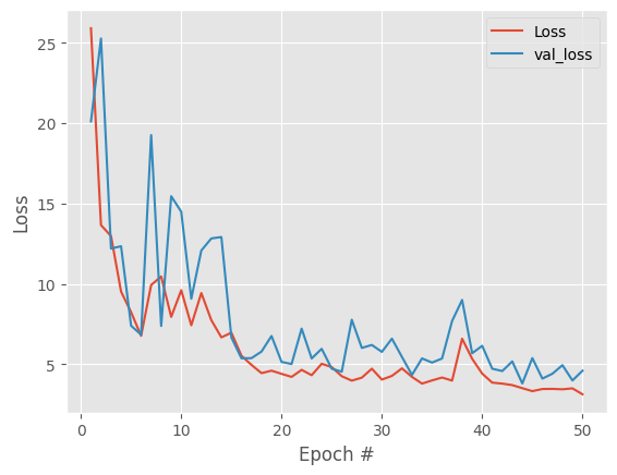
decreasing the learning rate.
 1autoencoder = create_l2_noise_autoencoder(
 2    neurons,
 3    train_data.shape[1],
 4    l2=1e-5,
 5    noise_std=0.1
 6)
 7
 8optimizer = tf.keras.optimizers.Adam(learning_rate=3e-4)
 9autoencoder.compile(
10    optimizer=optimizer,
11    loss='mean_squared_error'
12)
13
14H = autoencoder.fit(
15    train_data,
16    train_data,
17    validation_data=(test_data, test_data),
18    batch_size=32,
19    epochs=epochs,
20    verbose=1
21)
  1Epoch 1/50
  293/93 [==============================] - 3s 11ms/step - loss: 21.4099 - val_loss: 10.3221
  3Epoch 2/50
  493/93 [==============================] - 1s 10ms/step - loss: 8.7159 - val_loss: 7.0038
  5Epoch 3/50
  693/93 [==============================] - 1s 6ms/step - loss: 7.1138 - val_loss: 5.6221
  7Epoch 4/50
  893/93 [==============================] - 1s 11ms/step - loss: 5.6945 - val_loss: 5.7532
  9Epoch 5/50
 1093/93 [==============================] - 1s 11ms/step - loss: 4.9997 - val_loss: 4.4984
 11Epoch 6/50
 1293/93 [==============================] - 1s 13ms/step - loss: 4.5960 - val_loss: 4.6049
 13Epoch 7/50
 1493/93 [==============================] - 1s 11ms/step - loss: 4.3785 - val_loss: 4.9968
 15Epoch 8/50
 1693/93 [==============================] - 1s 11ms/step - loss: 3.9819 - val_loss: 4.3294
 17Epoch 9/50
 1893/93 [==============================] - 1s 12ms/step - loss: 3.8565 - val_loss: 3.8351
 19Epoch 10/50
 2093/93 [==============================] - 1s 8ms/step - loss: 3.8272 - val_loss: 4.0886
 21Epoch 11/50
 2293/93 [==============================] - 1s 6ms/step - loss: 3.6578 - val_loss: 3.8850
 23Epoch 12/50
 2493/93 [==============================] - 1s 13ms/step - loss: 4.0234 - val_loss: 4.2146
 25Epoch 13/50
 2693/93 [==============================] - 1s 16ms/step - loss: 3.6233 - val_loss: 3.9427
 27Epoch 14/50
 2893/93 [==============================] - 1s 9ms/step - loss: 3.7437 - val_loss: 4.0461
 29Epoch 15/50
 3093/93 [==============================] - 1s 13ms/step - loss: 3.3131 - val_loss: 3.2467
 31Epoch 16/50
 3293/93 [==============================] - 1s 6ms/step - loss: 3.0702 - val_loss: 3.2461
 33Epoch 17/50
 3493/93 [==============================] - 1s 10ms/step - loss: 3.0544 - val_loss: 3.3153
 35Epoch 18/50
 3693/93 [==============================] - 1s 14ms/step - loss: 3.4376 - val_loss: 4.1842
 37Epoch 19/50
 3893/93 [==============================] - 1s 10ms/step - loss: 3.2297 - val_loss: 3.2080
 39Epoch 20/50
 4093/93 [==============================] - 1s 11ms/step - loss: 2.8850 - val_loss: 3.1777
 41Epoch 21/50
 4293/93 [==============================] - 1s 12ms/step - loss: 2.8051 - val_loss: 2.9751
 43Epoch 22/50
 4493/93 [==============================] - 1s 11ms/step - loss: 2.7137 - val_loss: 3.0658
 45Epoch 23/50
 4693/93 [==============================] - 1s 10ms/step - loss: 2.8133 - val_loss: 3.3787
 47Epoch 24/50
 4893/93 [==============================] - 1s 10ms/step - loss: 3.5090 - val_loss: 3.1847
 49Epoch 25/50
 5093/93 [==============================] - 1s 9ms/step - loss: 2.7666 - val_loss: 3.1180
 51Epoch 26/50
 5293/93 [==============================] - 1s 13ms/step - loss: 2.7511 - val_loss: 3.0354
 53Epoch 27/50
 5493/93 [==============================] - 1s 12ms/step - loss: 2.9722 - val_loss: 3.0035
 55Epoch 28/50
 5693/93 [==============================] - 1s 12ms/step - loss: 2.7227 - val_loss: 3.0772
 57Epoch 29/50
 5893/93 [==============================] - 1s 13ms/step - loss: 2.6147 - val_loss: 2.7778
 59Epoch 30/50
 6093/93 [==============================] - 1s 12ms/step - loss: 2.5109 - val_loss: 3.0036
 61Epoch 31/50
 6293/93 [==============================] - 1s 13ms/step - loss: 2.6248 - val_loss: 3.1231
 63Epoch 32/50
 6493/93 [==============================] - 1s 9ms/step - loss: 2.5655 - val_loss: 3.0635
 65Epoch 33/50
 6693/93 [==============================] - 1s 12ms/step - loss: 2.5141 - val_loss: 2.8732
 67Epoch 34/50
 6893/93 [==============================] - 1s 14ms/step - loss: 2.8016 - val_loss: 2.9756
 69Epoch 35/50
 7093/93 [==============================] - 1s 11ms/step - loss: 2.7626 - val_loss: 3.0096
 71Epoch 36/50
 7293/93 [==============================] - 1s 11ms/step - loss: 2.8892 - val_loss: 3.1106
 73Epoch 37/50
 7493/93 [==============================] - 1s 11ms/step - loss: 2.7845 - val_loss: 2.9397
 75Epoch 38/50
 7693/93 [==============================] - 1s 12ms/step - loss: 2.4996 - val_loss: 3.1788
 77Epoch 39/50
 7893/93 [==============================] - 1s 13ms/step - loss: 2.4722 - val_loss: 2.7988
 79Epoch 40/50
 8093/93 [==============================] - 1s 10ms/step - loss: 2.3880 - val_loss: 2.6952
 81Epoch 41/50
 8293/93 [==============================] - 1s 10ms/step - loss: 2.3410 - val_loss: 2.6565
 83Epoch 42/50
 8493/93 [==============================] - 1s 10ms/step - loss: 2.3656 - val_loss: 3.5490
 85Epoch 43/50
 8693/93 [==============================] - 1s 11ms/step - loss: 3.1682 - val_loss: 2.7707
 87Epoch 44/50
 8893/93 [==============================] - 1s 11ms/step - loss: 2.5004 - val_loss: 2.7223
 89Epoch 45/50
 9093/93 [==============================] - 1s 12ms/step - loss: 2.4328 - val_loss: 2.6165
 91Epoch 46/50
 9293/93 [==============================] - 1s 10ms/step - loss: 2.2923 - val_loss: 2.8844
 93Epoch 47/50
 9493/93 [==============================] - 1s 11ms/step - loss: 2.4613 - val_loss: 2.7295
 95Epoch 48/50
 9693/93 [==============================] - 1s 9ms/step - loss: 2.3293 - val_loss: 2.6597
 97Epoch 49/50
 9893/93 [==============================] - 1s 13ms/step - loss: 2.2488 - val_loss: 2.5629
 99Epoch 50/50
10093/93 [==============================] - 1s 13ms/step - loss: 2.2132 - val_loss: 2.5368
1plt.style.use("ggplot")
2N = len(H.history["loss"])
3plt.plot(np.arange(1, N + 1), H.history["loss"], label="Loss")
4plt.plot(np.arange(1, N + 1), H.history["val_loss"], label="val_loss")
5plt.xlabel("Epoch #")
6plt.ylabel("Loss")
7plt.legend()
8plt.show()

extract and save bottleneck
1hidden_layer_array = np.array(hidden_layer_values)
2hidden_layer_df = pd.DataFrame(hidden_layer_array, columns=[f'Autoencoder_{i}' for i in range(hidden_layer_array.shape[1])])
3csv_output_path = 'hidden_layer.docker.1024.4.hidden50.earlystop.fixPreprocessing.csv'
4hidden_layer_df.to_csv(csv_output_path, index=False)
1csv_output_path = 'hidden_layer.docker.1024.4.hidden50.fixPreprocessing.csv'
2hidden_layer_df.to_csv(csv_output_path, index=False)
add the info to the SCE object
1autoencoder.df <- read.csv( 'hidden_layer.docker.1024.4.hidden50.fixPreprocessing.csv' )
2rownames(autoencoder.df) <- colnames(sce)
3reducedDim( sce, 'AE_50' ) <- autoencoder.df
now plot the results
1plotReducedDim( sce, dimred = 'AE_50', colour_by='clusters' )
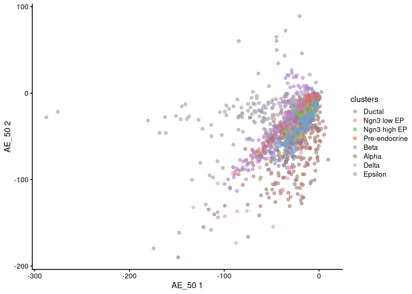
We see something now, it would be interesting to check the rest of dimensions since the neurons of the bottleneck are not arranged by relevance as the PCs.
let's do a tSNE
1sce <- runTSNE( sce, dimred = 'AE_50', name = 'TSNE_AE' )
2plotReducedDim( sce, dimred = 'TSNE_AE', colour_by='clusters' )
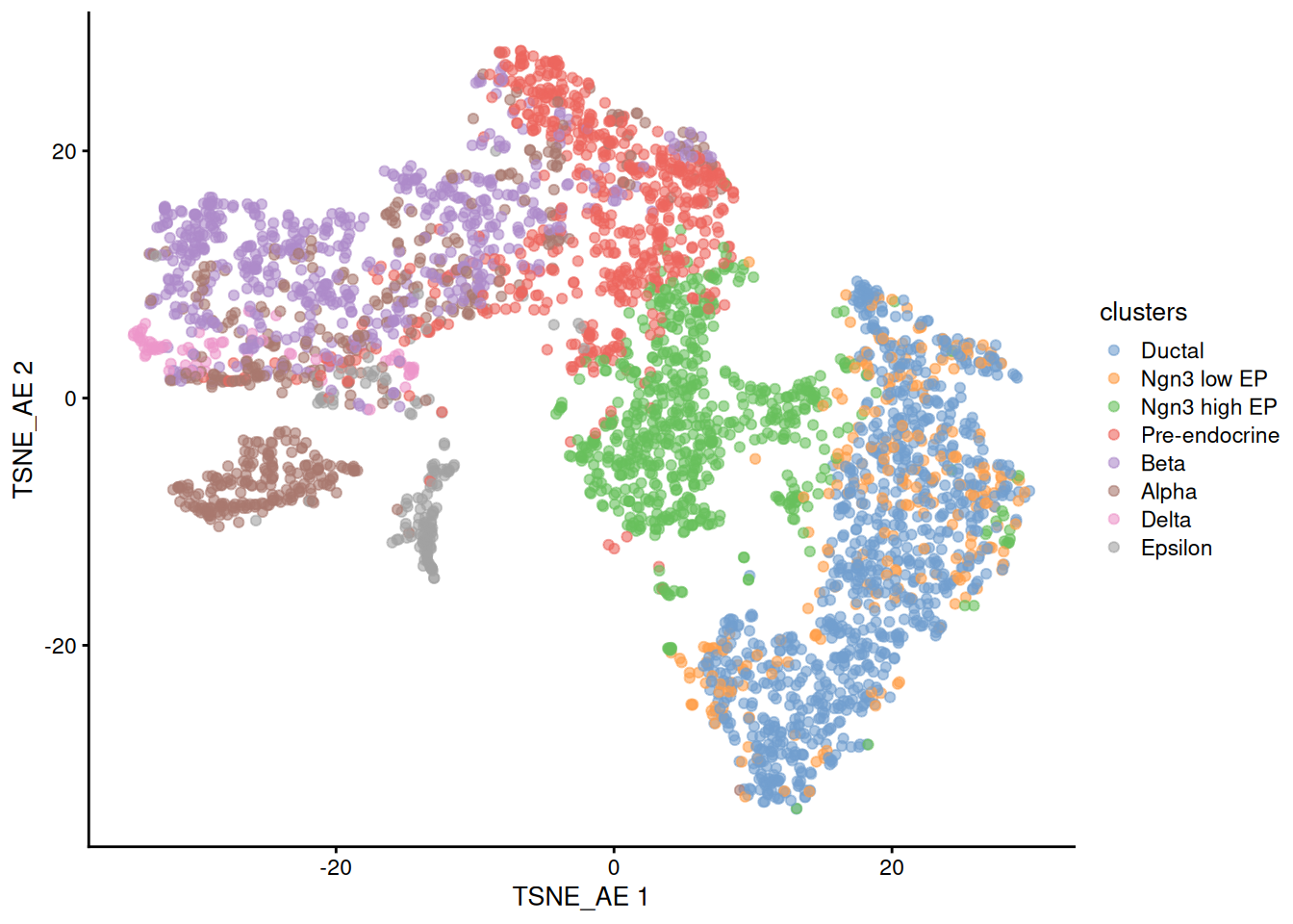
and UMAP
1sce <- runUMAP( sce, dimred = 'AE_50', name = 'UMAP_AE' )
2plotReducedDim( sce, dimred = 'UMAP_AE', colour_by='clusters' )
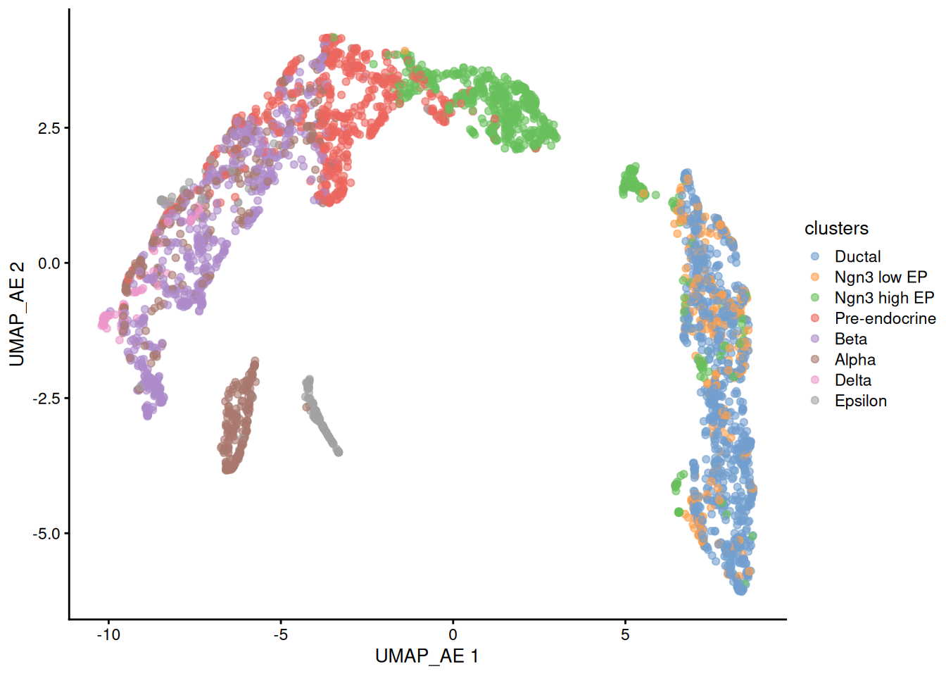
The original UMAP is nicer, but we start to see something in this plot.
Let's try to improve our autoencoder training adding early stopping to prevent overfitting (although it did not seem to be present).
Early stopping is a regularization technique that halts training when the model stops improving, it is useful to prevent overfitting.
Patience defines how many consecutive epochs with no sufficient improvement are allowed before training is stopped.
min_delta specifies the minimum change in the monitored metric that qualifies as an improvement
1from tensorflow.keras.callbacks import EarlyStopping
2early_stop = EarlyStopping(
3    monitor='val_loss',
4    patience=3,
5    min_delta=1e-2,
6    restore_best_weights=True,
7    verbose=1
8)
 1autoencoder = create_l2_noise_autoencoder(
 2    neurons,
 3    train_data.shape[1],
 4    l2=1e-5,
 5    noise_std=0.1
 6)
 7
 8optimizer = tf.keras.optimizers.Adam(learning_rate=3e-4)
 9autoencoder.compile(
10    optimizer=optimizer,
11    loss='mean_squared_error'
12)
1H = autoencoder.fit(
2    x=train_data,
3    y=train_data,
4    validation_data=(test_data, test_data),
5    batch_size=32,
6    epochs=epochs,
7    callbacks=[early_stop],
8    verbose=1
9)
 1Epoch 1/50
 293/93 [==============================] - 3s 13ms/step - loss: 24.5211 - val_loss: 11.7137
 3Epoch 2/50
 493/93 [==============================] - 1s 8ms/step - loss: 9.1473 - val_loss: 13.0406
 5Epoch 3/50
 693/93 [==============================] - 1s 11ms/step - loss: 7.6864 - val_loss: 6.1292
 7Epoch 4/50
 893/93 [==============================] - 1s 7ms/step - loss: 5.7401 - val_loss: 5.3677
 9Epoch 5/50
1093/93 [==============================] - 1s 15ms/step - loss: 5.0120 - val_loss: 4.6072
11Epoch 6/50
1293/93 [==============================] - 1s 10ms/step - loss: 4.4506 - val_loss: 4.4444
13Epoch 7/50
1493/93 [==============================] - 1s 13ms/step - loss: 4.1622 - val_loss: 4.9327
15Epoch 8/50
1693/93 [==============================] - 1s 13ms/step - loss: 4.5532 - val_loss: 4.3296
17Epoch 9/50
1893/93 [==============================] - 1s 12ms/step - loss: 4.1559 - val_loss: 3.8712
19Epoch 10/50
2093/93 [==============================] - 1s 12ms/step - loss: 4.0565 - val_loss: 4.3901
21Epoch 11/50
2293/93 [==============================] - 1s 10ms/step - loss: 3.8009 - val_loss: 3.8640
23Epoch 12/50
2493/93 [==============================] - 1s 8ms/step - loss: 4.2816 - val_loss: 3.7222
25Epoch 13/50
2693/93 [==============================] - 1s 13ms/step - loss: 3.3293 - val_loss: 3.5383
27Epoch 14/50
2893/93 [==============================] - 1s 12ms/step - loss: 3.3962 - val_loss: 3.3154
29Epoch 15/50
3093/93 [==============================] - 1s 11ms/step - loss: 3.1298 - val_loss: 4.0492
31Epoch 16/50
3293/93 [==============================] - 1s 9ms/step - loss: 3.2114 - val_loss: 3.5338
33Epoch 17/50
3492/93 [============================>.] - ETA: 0s - loss: 3.0252Restoring model weights from the end of the best epoch: 14.
3593/93 [==============================] - 1s 11ms/step - loss: 3.0218 - val_loss: 3.5410
36Epoch 17: early stopping
1plt.style.use("ggplot")
2N = len(H.history["loss"])
3plt.plot(np.arange(1, N + 1), H.history["loss"], label="Loss")
4plt.plot(np.arange(1, N + 1), H.history["val_loss"], label="val_loss")
5plt.xlabel("Epoch #")
6plt.ylabel("Loss")
7plt.legend()
8plt.show()
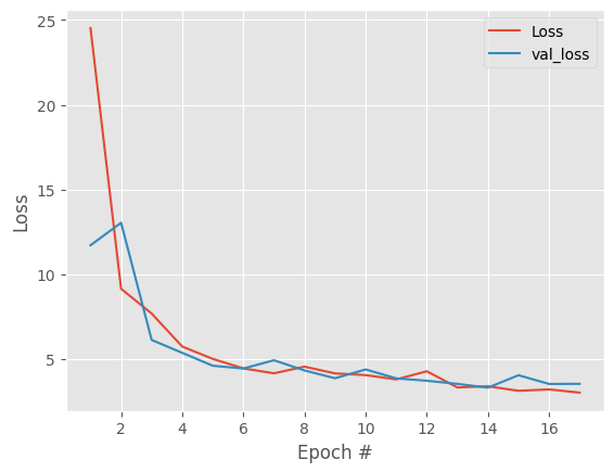
extract and save the bottleneck
1hidden_layer_array = np.array(hidden_layer_values)
2hidden_layer_df = pd.DataFrame(hidden_layer_array, columns=[f'Autoencoder_{i}' for i in range(hidden_layer_array.shape[1])])
3csv_output_path = 'hidden_layer.docker.1024.4.hidden50.earlystop.fixPreprocessing.csv'
4hidden_layer_df.to_csv(csv_output_path, index=False)
add the information to the SCE
1autoencoder.df <- read.csv( 'hidden_layer.docker.1024.4.hidden50.earlystop.fixPreprocessing.csv' )
2rownames(autoencoder.df) <- colnames(sce)
3reducedDim( sce, 'AE_50_early' ) <- autoencoder.df
now plot the results
1plotReducedDim( sce, dimred = 'AE_50_early', colour_by='clusters' )
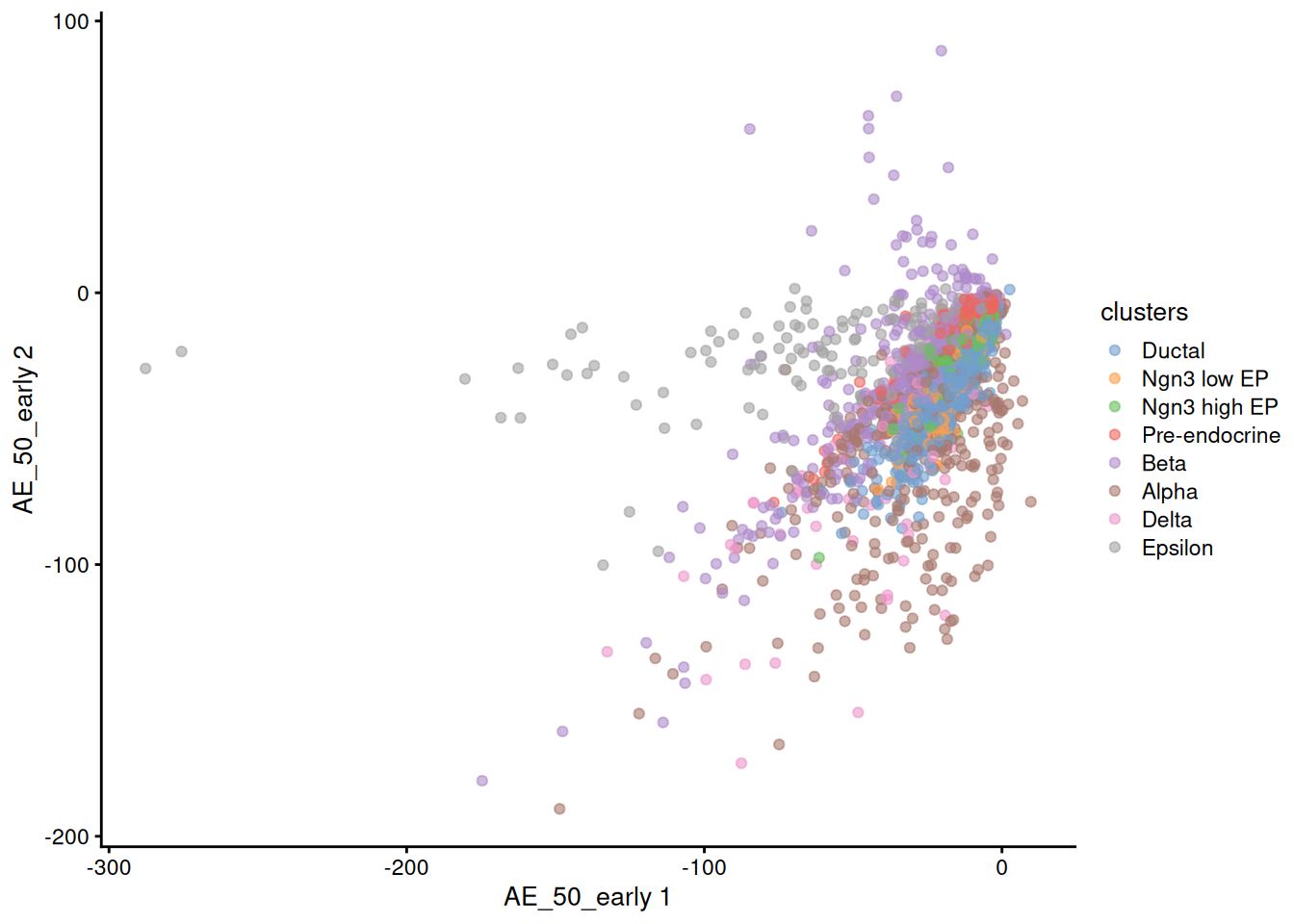
Very similar results, let's see the tSNE
1sce <- runTSNE( sce, dimred = 'AE_50_early', name = 'TSNE_AE2' )
2plotReducedDim( sce, dimred = 'TSNE_AE2', colour_by='clusters' )
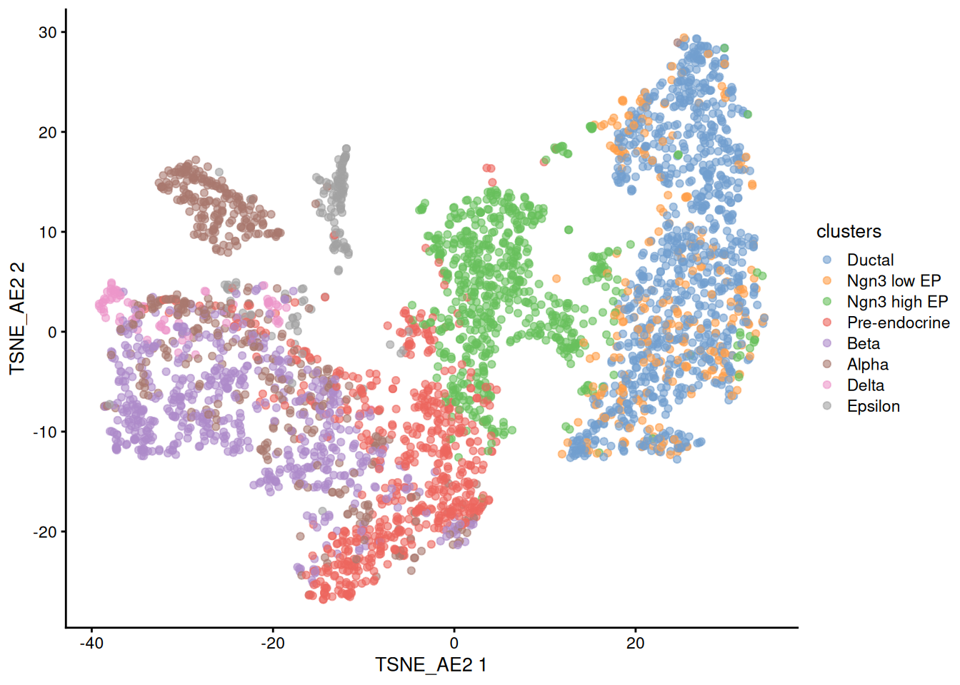
and UMAP
1sce <- runUMAP( sce, dimred = 'AE_50_early', name = 'UMAP_AE2' )
2plotReducedDim( sce, dimred = 'UMAP_AE2', colour_by='clusters' )
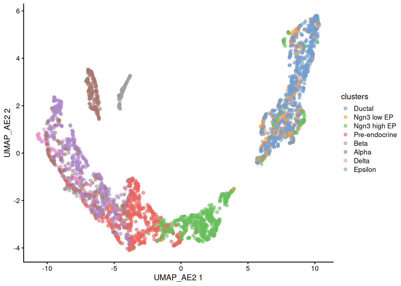
Again a plot that shows a similar cell organization to the original UMAP although the original representation is still better.
Conclusions
There are several types of autoencoders, today we used the most basic implementation. The most widely used autoencoder type in bioinformatics is the variational autoencoder (VAE), which learns a probability distribution rather than a discrete set of values in the latent space. This probabilistic latent space is well suited to noisy, sparse biological data and supports tasks such as batch correction and data generation. Examples of VAE-based models range from scVI to the more recently described FAVA (Functional Associations using Variational Autoencoders).
Take home messages
- Autoencoders can efficiently compress single cell expression data even with this quick and non-optimal configuaration
- Autoencoders are fast and scalable, making them well suited to the constant increase in dataset size in the single-cell field
- Learning how autoencoders work helps you understand the internal mechanisms of many deep-learning tools, enabling you to better evaluate and interpret their outputs on your own datasets