Find Marker Genes Using Effect Size
1suppressMessages({
2  library(scRNAseq)
3  library(scater)
4  library(scran)
5  library(org.Mm.eg.db)
6  library(VennDiagram)
7  library(wesanderson)
8})
It has been a while since I wrote my last post, for today I decided to focus on something that has been in mind for a long time but never found the time of properly testing, marker gene selection. Cluster marker genes can be defined as genes that drive separation between clusters and allow us to assign biological meaning to each cluster. The most immediate approach is to perform differential gene expression between clusters. Strong DEGs are more likely to be driving the separation of the clusters.
Like many aspects of single cell analysis, things are not as easy as they may seem. Most DE analysis methods treat cells as independent observations, however this is not really accurate when cells are derived from the same biological sample (i.e., cell culture, animal or patient) and therefore the sample-to-sample variability is not properly addressed.
This point becomes more relevant when you think about the typical single cell workflow: cluster cells based on gene expression profiles and then find markers genes to identify/annotate those clusters. This is known as the circularity issue / double deeping / data dredging / fishing / data snooping:
- Make hypotheses based on your data.
- Test them on the same data
- Statistical tests cannot properly control Type I error rate on these situations
Many tutorials and packages perform marker gene selection using classical statistical test like Wilcoxon or t-test. The common assumption is that ranking genes by the P-value, although inflated, is a good enough approach to find marker genes.
The OSCA book chapter on marker gene detection proposes a different approach based on effect size that I think is better. The idea is ranking the genes by a measure of the expression difference, fold change would be an example, to select as marker genes the ones with the biggest difference in expression, instead of the most significant ones.
To test this idea, we will use a couple of datasets from the scRNAseq bioconductor package with annotated cell types. Cell types will be used as a proxy of cell cluster allowing us to check the quality of the selected markers.
Zeisel dataset
- ~3,000 cells, mouse brain (cortex + hippocampus)
- Comes with a level1class annotation (7 broad cell types: pyramidal neurons, interneurons, microglia, oligodendrocytes, astrocytes, endothelial, ependymal)
1sce.zeisel <- ZeiselBrainData()
check data
1sce.zeisel
 1## class: SingleCellExperiment
 2## dim: 20006 3005
 3## metadata(0):
 4## assays(1): counts
 5## rownames(20006): Tspan12 Tshz1 ... mt-Rnr1 mt-Nd4l
 6## rowData names(1): featureType
 7## colnames(3005): 1772071015_C02 1772071017_G12 ... 1772066098_A12
 8##   1772058148_F03
 9## colData names(9): tissue group # ... level1class level2class
10## reducedDimNames(0):
11## mainExpName: gene
12## altExpNames(2): repeat ERCC
Follow processing as described in OSCA book
1sce.zeisel <- aggregateAcrossFeatures(sce.zeisel,
2                                      id=sub("_loc[0-9]+$", "", rownames(sce.zeisel)))
3rowData(sce.zeisel)$Ensembl <- mapIds(org.Mm.eg.db,
4                                      keys=rownames(sce.zeisel), keytype="SYMBOL", column="ENSEMBL")
1## 'select()' returned 1:many mapping between keys and columns
 1stats <- perCellQCMetrics(sce.zeisel, subsets=list(
 2    Mt=rowData(sce.zeisel)$featureType=="mito"))
 3qc <- quickPerCellQC(stats, percent_subsets=c("altexps_ERCC_percent",
 4    "subsets_Mt_percent"))
 5sce.zeisel <- sce.zeisel[,!qc$discard]
 6set.seed(1000)
 7clusters <- quickCluster(sce.zeisel)
 8sce.zeisel <- computeSumFactors(sce.zeisel, cluster=clusters)
 9sce.zeisel <- logNormCounts(sce.zeisel)
10dec.zeisel <- modelGeneVarWithSpikes(sce.zeisel, "ERCC")
11top.hvgs <- getTopHVGs(dec.zeisel, prop=0.1)
12
13sce.zeisel <- denoisePCA(sce.zeisel, technical=dec.zeisel, subset.row=top.hvgs)
14sce.zeisel <- runTSNE(sce.zeisel, dimred="PCA")
15sce.zeisel <- runUMAP(sce.zeisel, dimred="PCA")
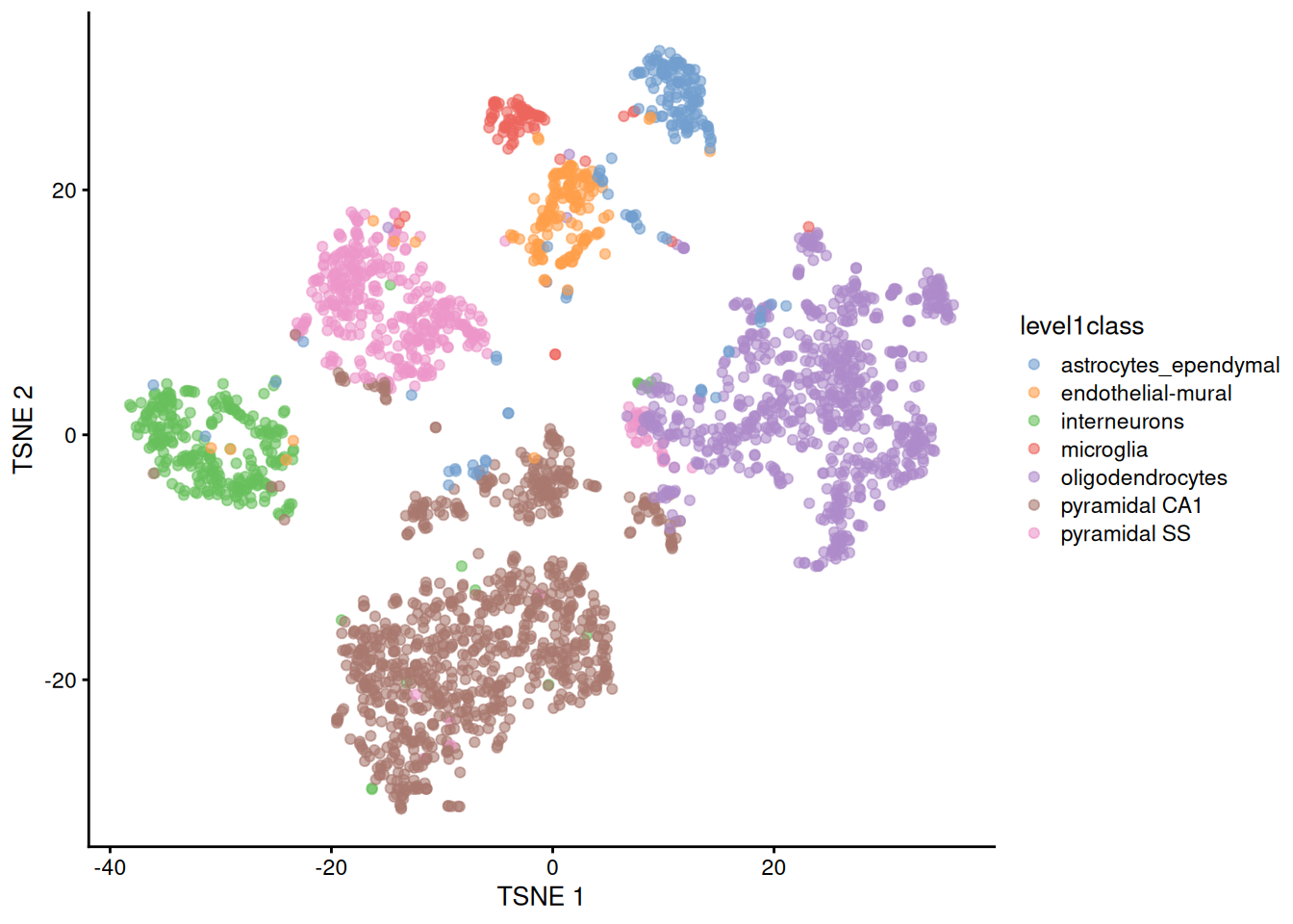
1plotTSNE( sce.zeisel, colour_by = 'level1class' )
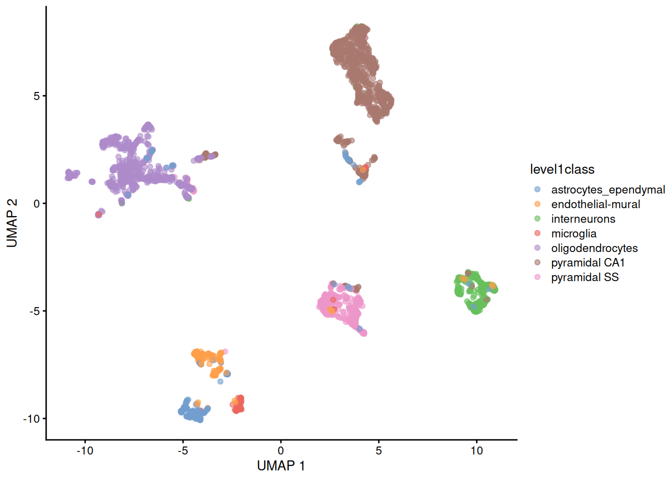
1plotUMAP( sce.zeisel, colour_by = 'level1class' )
P-value
We will use the findMarkers function from scran package (very similar to the seurat's function with the same name, or rank_genes_groups from scanpy. It defaults to a t-test, use the test.type argument to change it:
- "t", defaults to a Welch t-tests
- "wilcox", pairwise Wilcoxon rank sum test
- "binom", pairwise binomial tests
it works by comparing each cluster/cell type/ group of cells to every other independently and summarizing the results as follows
| pval.type | Question being asked | Best for |
|---|---|---|
any (default) |
Does this gene separate the cluster from some other cluster? | Marker combinations, general clustering QC |
some |
Does this gene separate the cluster from most other clusters? | Compromise, robust to one similar neighboring cluster |
all |
Does this gene separate the cluster from every other cluster? | Canonical, cluster-exclusive markers; best with well-separated, non-redundant clusters (like Zeisel's 7 broad types) |
We use pairwise comparisons rather than comparing each cell type to all other cells because the latter approach is sensitive to the population composition while pairwise comparisons naturally provide more information to interpret cell population structure.
all
We start with this option which will find genes completely specific to the selected cell type
1markers <- findMarkers( sce.zeisel, groups = sce.zeisel$level1class, direction="up", pval.type = 'all' )
2names(markers)
1## [1] "astrocytes_ependymal" "endothelial-mural"    "interneurons"
2## [4] "microglia"            "oligodendrocytes"     "pyramidal CA1"
3## [7] "pyramidal SS"
we will focus on the astrocytes
1marker.set <- markers[["astrocytes_ependymal"]]
2head(marker.set)
 1## DataFrame with 6 rows and 9 columns
 2##            p.value         FDR summary.logFC logFC.endothelial-mural
 3##          <numeric>   <numeric>     <numeric>               <numeric>
 4## Aqp4   9.44070e-65 1.87294e-60       4.41445                 4.44859
 5## Cldn10 4.50175e-59 4.46552e-55       3.31739                 3.29126
 6## Clu    3.59649e-53 2.37836e-49       5.29763                 5.20606
 7## Ntsr2  1.45913e-51 7.23694e-48       3.19148                 3.25929
 8## Aldoc  3.37659e-50 1.33976e-46       3.89718                 4.06435
 9## Mt2    1.69515e-49 5.60501e-46       4.09232                 3.73900
10##        logFC.interneurons logFC.microglia logFC.oligodendrocytes
11##                 <numeric>       <numeric>              <numeric>
12## Aqp4              4.66310         4.41445                4.42523
13## Cldn10            3.44648         3.31739                3.24379
14## Clu               3.60647         5.29763                5.26771
15## Ntsr2             3.42934         3.19148                3.23559
16## Aldoc             3.88556         3.89718                4.07250
17## Mt2               4.66218         4.09232                4.31965
18##        logFC.pyramidal CA1 logFC.pyramidal SS
19##                  <numeric>          <numeric>
20## Aqp4               4.58979            4.62308
21## Cldn10             3.20419            3.37479
22## Clu                4.83699            4.13796
23## Ntsr2              3.31741            3.39548
24## Aldoc              4.29262            4.17278
25## Mt2                4.64615            4.73419
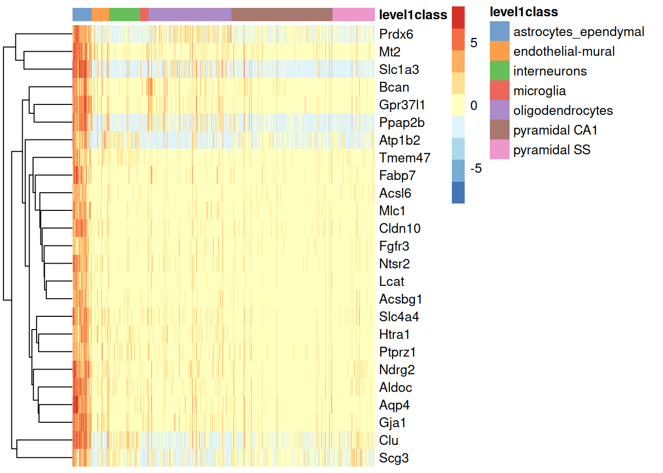
and use the top 25 genes
1top.markers <- rownames(marker.set)[1:25]
2plotHeatmap( sce.zeisel,
3             features=top.markers,
4             order_columns_by="level1class",
5             center=TRUE
6           )
1plotGroupedHeatmap( sce.zeisel,
2                    features=top.markers,
3                    group="level1class",
4                    center=TRUE
5                  )
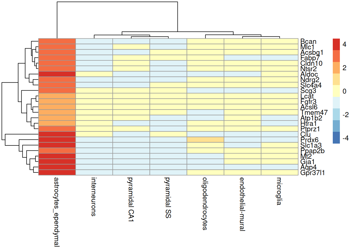
Most are strong, literature-validated astrocyte markers:
- Aqp4: aquaporin-4, the textbook pan-astrocyte marker, especially enriched at perivascular endfeet
- Slc1a3 (GLAST): classic astrocytic glutamate transporter, used in countless astrocyte-labeling mouse lines
- Gja1 (Connexin-43): canonical astrocyte gap-junction protein
- Atp1b2 (AMOG): long-established astrocyte-specific Na+/K+-ATPase subunit
- Slc4a4 (NBCe1): canonical astrocyte bicarbonate transporter
- Ndrg2: specifically expressed in astrocytes of the brain and regarded as a novel, reliable astrocytic marker
- Fabp7 (BLBP): classic radial glia/astrocyte marker
- Mlc1, Gpr37l1, Ptprz1, Bcan, Fgfr3: repeatedly reported as astrocyte- or astrocyte/OPC-enriched genes in cortical scRNA-seq atlases
- Ntsr2, Aldoc, Htra1, Clu, Cldn10, Prdx6, Acsbg1, Lcat: consistently top astrocyte-enriched genes in mouse brain scRNA-seq references (including this Zeisel dataset's own original marker panel)
Worth a second look genes
- Mt2 (metallothionein 2): a general stress-response/metal-binding gene; enriched in astrocytes but less specific, since it can be induced in reactive states across cell types
- Scg3 (secretogranin III): stands out; typically associated with neuroendocrine secretory granules rather than astrocyte biology. Could be a real but less-documented signal, low-level ambient/background contamination in droplet-based data, or an artifact of one particularly distinctive pairwise comparison driving its
some-type combined significance. - Tmem47: reported in some astrocyte transcriptomic studies but far less characterized than the others; plausible but not a "textbook" marker
some
We try now this option which will find genes enriched but possible not completely specific to the selected cell type
1markers <- findMarkers( sce.zeisel, groups = sce.zeisel$level1class, direction="up", pval.type = 'some' )
2names(markers)
1## [1] "astrocytes_ependymal" "endothelial-mural"    "interneurons"
2## [4] "microglia"            "oligodendrocytes"     "pyramidal CA1"
3## [7] "pyramidal SS"
1marker.set <- markers[["astrocytes_ependymal"]]
2head(marker.set)
 1## DataFrame with 6 rows and 9 columns
 2##             p.value          FDR summary.logFC logFC.endothelial-mural
 3##           <numeric>    <numeric>     <numeric>               <numeric>
 4## Apoe   8.97746e-129 1.78104e-124       5.36624                 5.34228
 5## Slc1a3 2.06515e-114 2.04852e-110       5.58194                 5.05382
 6## Mt1    3.02832e-108 2.00262e-104       5.45505                 4.20940
 7## Clu    4.11625e-107 2.04156e-103       5.20606                 5.20606
 8## Gja1   6.65536e-103  2.64072e-99       4.29960                 3.90276
 9## Atp1a2 1.74957e-102  5.78495e-99       6.04912                 3.33541
10##        logFC.interneurons logFC.microglia logFC.oligodendrocytes
11##                 <numeric>       <numeric>              <numeric>
12## Apoe              6.30921        0.340815                5.36624
13## Slc1a3            5.71075        4.781766                4.58897
14## Mt1               5.30828        3.585627                3.79059
15## Clu               3.60647        5.297635                5.26771
16## Gja1              4.70872        3.960957                4.29960
17## Atp1a2            6.31122        4.569073                4.91068
18##        logFC.pyramidal CA1 logFC.pyramidal SS
19##                  <numeric>          <numeric>
20## Apoe               6.05976            6.14838
21## Slc1a3             5.58194            5.62350
22## Mt1                5.45505            5.44808
23## Clu                4.83699            4.13796
24## Gja1               4.56702            4.62901
25## Atp1a2             6.04912            5.70395
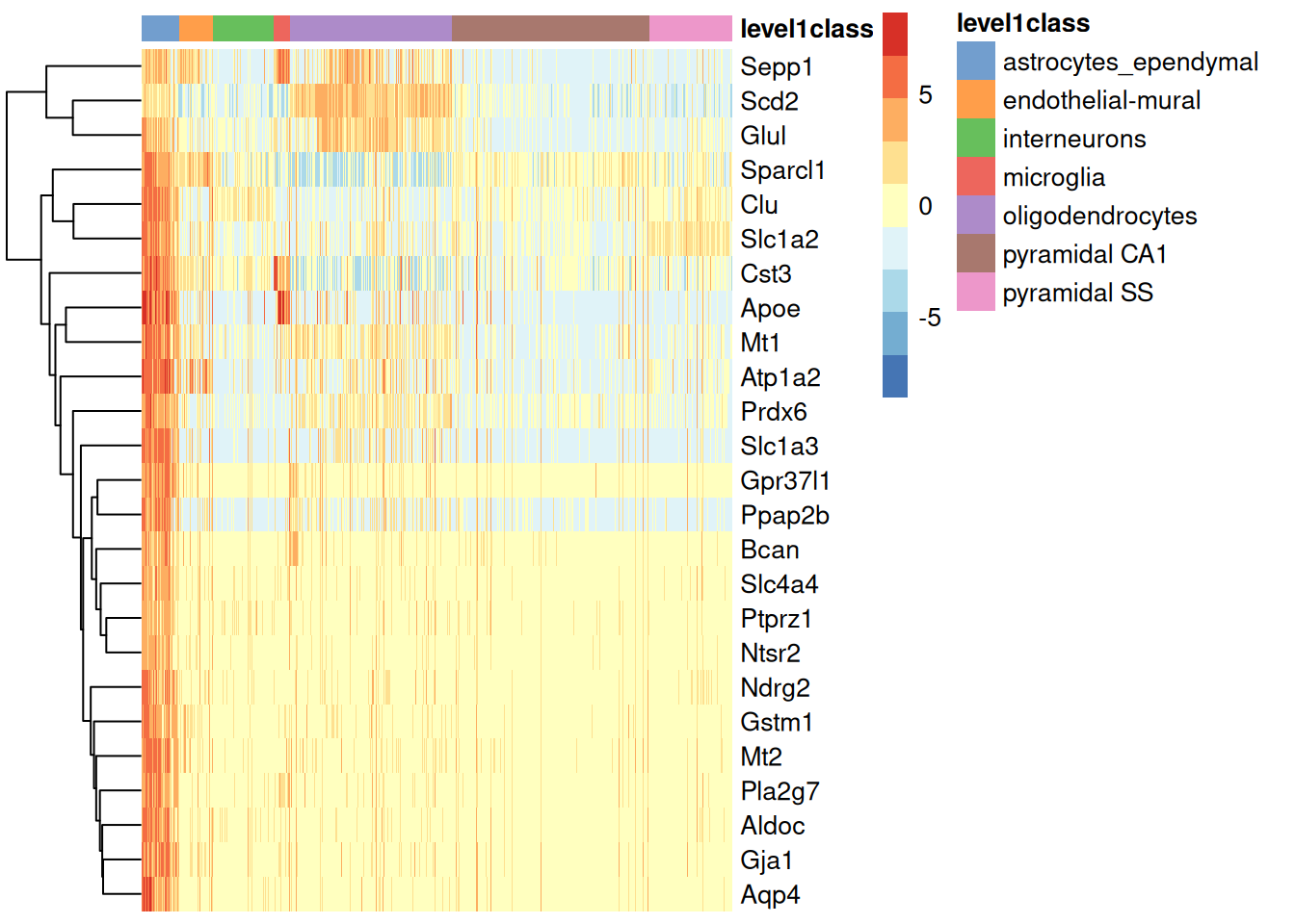
1top.markers.some <- rownames(marker.set)[1:25]
2plotHeatmap( sce.zeisel,
3             features=top.markers.some,
4             order_columns_by="level1class",
5             center=TRUE
6           )
1plotGroupedHeatmap( sce.zeisel,
2                    features=top.markers.some,
3                    group="level1class",
4                    center=TRUE
5                  )
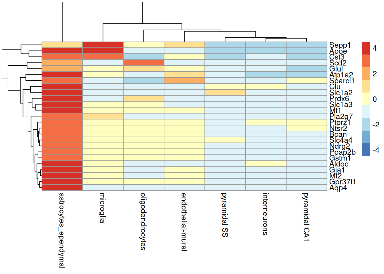
Most are strong, literature-validated astrocyte markers, including
several top-tier "textbook" genes not seen in the all-type list:
- Apoe: the major lipid/cholesterol transport protein secreted by astrocytes in the CNS; one of the most-cited astrocyte identity genes in the field
- Slc1a3 (GLAST), Slc1a2 (GLT-1/EAAT2): the two primary astrocytic glutamate transporters; Slc1a2 is arguably even more central to astrocyte identity than Slc1a3
- Gja1 (Connexin-43): canonical astrocyte gap-junction protein
- Atp1a2: canonical astrocyte-specific Na+/K+-ATPase alpha subunit
- Sparcl1 (Hevin): canonical astrocyte-secreted synaptogenic factor
- Glul: glutamine synthetase, arguably the textbook astrocyte enzyme, central to the glutamate-glutamine cycle
- Aqp4, Slc4a4, Ndrg2, Ptprz1, Ntsr2, Aldoc, Gpr37l1, Bcan, Prdx6, Ppap2b: repeatedly reported as astrocyte-enriched genes in cortical scRNA-seq atlases
Worth a second look because they are less classic:
- Mt1, Mt2 (metallothioneins): general stress-response/metal-binding genes; enriched in astrocytes but less specific, inducible in reactive states across cell types
- Pla2g7 (Lp-PLA2/PAFAH): more strongly associated in much of the literature with monocyte/macrophage/microglial biology than astrocytes; could reflect a genuine subpopulation, ambient RNA from nearby microglia, or a doublet effect
- Cst3 (cystatin C): fairly broadly expressed across glial and even non-neural tissue, so less specific than the top-tier genes above
- Sepp1 (Selenoprotein P): known astrocyte-secreted antioxidant protein; well documented but less famous than Glul
- Scd2, Gstm1: plausible astrocyte-enriched metabolic genes, fit the recurring lipid-metabolism theme, but less "textbook" than the top markers
Cohen's D
We now move to an analysis not based on P-values using the scoreMarkers function from scran package. To the best of my knowledge there is no equivalent in seurat or scanpy but you can try scranpy in Python (check my post on BiocPy: Bioconductor in Python).
As before, we will compare each cell type to each other independently but, instead of performing a statistical test it calculates several scores to quantify the differences in the expression distributions. Next, we will rank candidate markers based on one of these effect size summaries.
There are two main scores:
- The area under the curve (AUC) quantifies our ability to distinguish between two distributions in a pairwise comparison. The AUC represents the probability that a randomly chosen observation from the cell type of interest is greater than a randomly chosen observation from the other cell type.
- Cohen’s d is a standardized log-fold change that measures effect size where the difference in the mean log-expression between groups is scaled by the average standard deviation across groups. Same idea as the log-fold change but log-fold change tells you the magnitude of the difference while effect size tells you the reliability/separability of the difference. A good marker gene ideally has both, large mean difference and non-overlapping distributions.
Following calculation, the pairwise scores are aggregated using typical summary statistics like the mean, median or maximum. We will focus on the following two:
- The median effect size, a large positive value indicates that the gene is upregulated in the cell type of interest compared to the average of the other ones. The median provides greater robustness to outliers than the mean.
- The minimum value is the most stringent summary for identifying upregulated genes, as a large value indicates that the gene is upregulated in the cell type of interest compared to all the other ones.
median
We start with the mean that evaluates differences to most but not all cell types in the dataset.
1marker.info <- scoreMarkers( sce.zeisel, groups = sce.zeisel$level1class )
2names(marker.info)
1## [1] "astrocytes_ependymal" "endothelial-mural"    "interneurons"
2## [4] "microglia"            "oligodendrocytes"     "pyramidal CA1"
3## [7] "pyramidal SS"
1chosen <- marker.info[["astrocytes_ependymal"]]
2ordered <- chosen[order(chosen$median.logFC.cohen,decreasing=TRUE),]
3head(ordered)
 1## DataFrame with 6 rows and 19 columns
 2##         self.average other.average self.detected other.detected
 3##            <numeric>     <numeric>     <numeric>      <numeric>
 4## Slc1a3       5.97823      0.754770      0.983240       0.265159
 5## Apoe         6.56046      1.632683      1.000000       0.351455
 6## Gja1         4.85359      0.508912      0.983240       0.214221
 7## Clu          6.21790      1.492429      0.994413       0.618106
 8## Gpr37l1      4.86027      0.453929      0.972067       0.158365
 9## Pla2g7       4.39260      0.619424      0.944134       0.239782
10##         mean.logFC.cohen min.logFC.cohen median.logFC.cohen max.logFC.cohen
11##                <numeric>       <numeric>          <numeric>       <numeric>
12## Slc1a3           3.67601        2.712489            3.68077         4.60039
13## Apoe             3.37960        0.168621            3.66780         5.04830
14## Gja1             3.58473        2.813154            3.65425         4.36901
15## Clu              3.47752        3.007695            3.59248         3.63657
16## Gpr37l1          3.43198        2.785091            3.40197         4.20804
17## Pla2g7           3.06031        1.386777            3.33164         3.64626
18##         rank.logFC.cohen  mean.AUC   min.AUC median.AUC   max.AUC  rank.AUC
19##                <integer> <numeric> <numeric>  <numeric> <numeric> <integer>
20## Slc1a3                 2  0.971184  0.941412   0.974113  0.987160         3
21## Apoe                   1  0.900640  0.495989   0.976723  0.994548         1
22## Gja1                   2  0.973603  0.954197   0.976803  0.987536         2
23## Clu                    1  0.976374  0.966779   0.977677  0.980761         1
24## Gpr37l1                2  0.963477  0.945269   0.963971  0.982537         4
25## Pla2g7                 2  0.943827  0.859332   0.960745  0.965692         5
26##         mean.logFC.detected min.logFC.detected median.logFC.detected
27##                   <numeric>          <numeric>             <numeric>
28## Slc1a3             2.030578          0.9313558              2.089780
29## Apoe               1.838217          0.1139562              1.963239
30## Gja1               2.378503          1.3997949              2.393263
31## Clu                0.817669          0.0474345              0.916262
32## Gpr37l1            2.708740          1.8132196              2.717976
33## Pla2g7             2.292453          0.4145697              2.539440
34##         max.logFC.detected rank.logFC.detected
35##                  <numeric>           <integer>
36## Slc1a3             3.05016                 211
37## Apoe               3.03333                 214
38## Gja1               3.72940                  70
39## Clu                1.54091                1262
40## Gpr37l1            3.78132                  63
41## Pla2g7             3.19337                 114
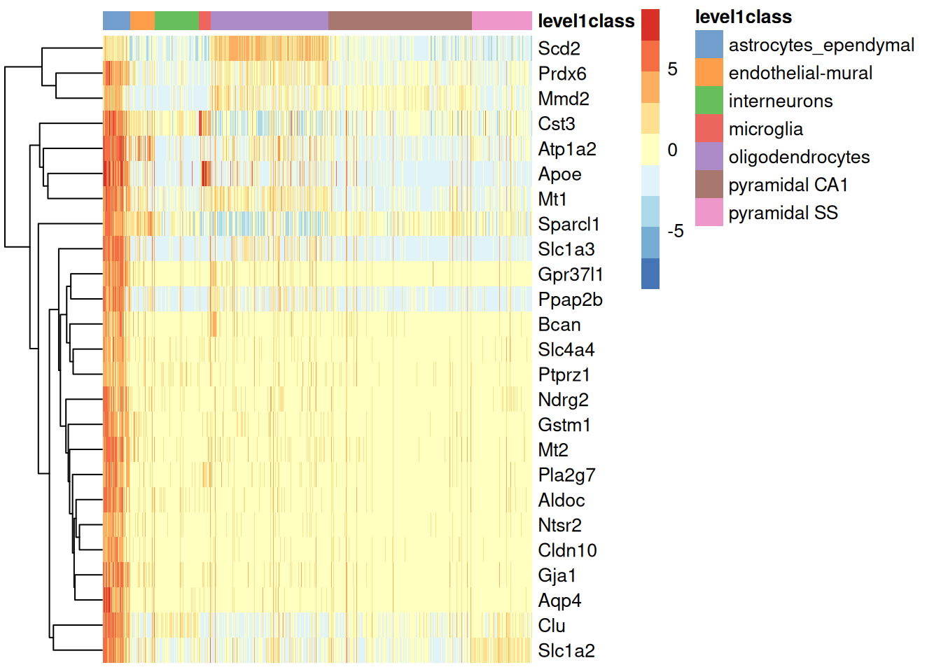
1top.cohen.markers <- rownames(ordered)[1:length(top.markers)]
2plotHeatmap( sce.zeisel,
3             features=top.cohen.markers,
4             order_columns_by="level1class",
5             center=TRUE
6           )
1plotGroupedHeatmap( sce.zeisel,
2                    features=top.cohen.markers,
3                    group="level1class",
4                    center=TRUE
5                  )
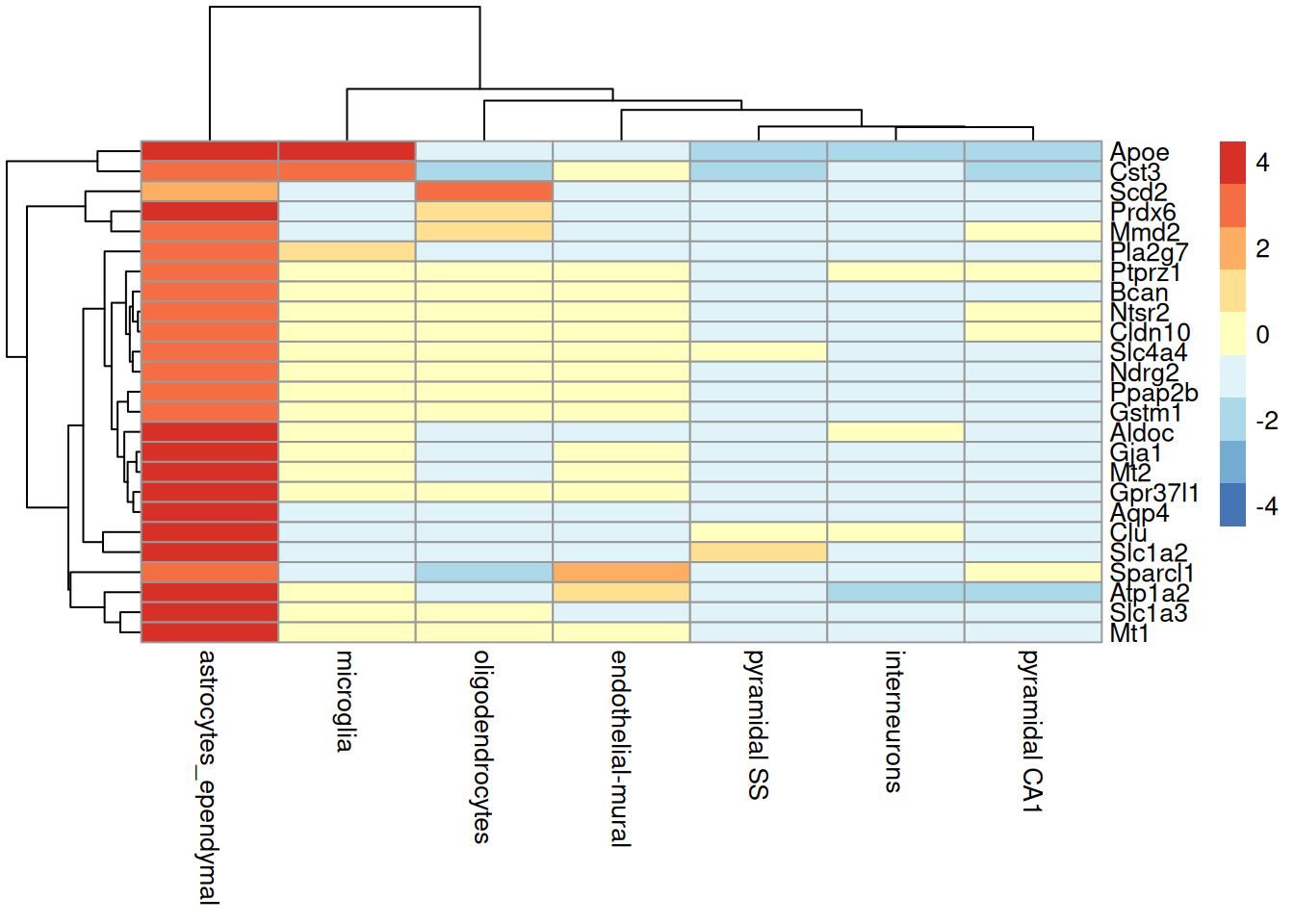
This list is very strong, possibly even more canonical than the findMarkers list, because it captures several extremely well-known astrocyte identity genes that didn't show up in the previous list.
Canonical, high-confidence astrocyte markers (new in this list)
- Apoe: the major lipid/cholesterol transport protein secreted by
astrocytes in the CNS; one of the most-cited astrocyte identity genes
in the field, notably absent from the
findMarkerstop-25 - Slc1a2 (GLT-1/EAAT2): the primary astrocytic glutamate transporter (arguably even more central to astrocyte identity than Slc1a3/GLAST), also missing from the earlier list
- Sparcl1 (Hevin): canonical astrocyte-secreted synaptogenic factor
- Atp1a2: canonical astrocyte-specific Na+/K+-ATPase alpha subunit (pairs with Atp1b2 from the earlier list)
These four alone are a strong sign that scoreMarkers's
median-Cohen's-d ranking is picking up genuinely central astrocyte
biology, not just statistically convenient genes.
Same genes/themes as the findMarkers list: Gstm1, Mt1 (paralog of
Mt2), Cst3: reasonable astrocyte-enriched genes, though Cst3
(cystatin C) is fairly broadly expressed across glial and even
non-neural tissue, so it's less specific than the top-tier genes above.
Scd2 fits the recurring lipid-metabolism theme (alongside Aldoc,
Sparcl1, Apoe): consistent with astrocytes' core role in lipid handling.
Worth double-checking with different lineage associations
- Pla2g7 (Lp-PLA2/PAFAH): a flag. In much of the literature, Pla2g7 is more strongly associated with monocyte/macrophage/microglial biology than astrocytes. Its presence here could reflect a genuine astrocyte-expressed subpopulation, ambient RNA from nearby microglia, or a doublet effect. Worth a violin/dot plot across all 7 cell types.
- Mmd2: "monocyte to macrophage differentiation-associated 2": similar concern; its name reflects a different original expression context, though some brain atlases do report low-level astrocyte enrichment. Same recommendation: check specificity directly.
min
Using the minium value, only gene upregulated in comparison to every other cell type will be detected.
1ordered <- chosen[order(chosen$min.logFC.cohen,decreasing=TRUE),]
2head(ordered)
 1## DataFrame with 6 rows and 19 columns
 2##         self.average other.average self.detected other.detected
 3##            <numeric>     <numeric>     <numeric>      <numeric>
 4## Clu          6.21790      1.492429      0.994413       0.618106
 5## Gja1         4.85359      0.508912      0.983240       0.214221
 6## Gpr37l1      4.86027      0.453929      0.972067       0.158365
 7## Aqp4         4.79917      0.271795      0.932961       0.113509
 8## Slc1a3       5.97823      0.754770      0.983240       0.265159
 9## Aldoc        4.54419      0.480026      0.916201       0.241445
10##         mean.logFC.cohen min.logFC.cohen median.logFC.cohen max.logFC.cohen
11##                <numeric>       <numeric>          <numeric>       <numeric>
12## Clu              3.47752         3.00770            3.59248         3.63657
13## Gja1             3.58473         2.81315            3.65425         4.36901
14## Gpr37l1          3.43198         2.78509            3.40197         4.20804
15## Aqp4             2.91641         2.74180            2.90287         3.12477
16## Slc1a3           3.67601         2.71249            3.68077         4.60039
17## Aldoc            2.67529         2.42491            2.62957         2.92491
18##         rank.logFC.cohen  mean.AUC   min.AUC median.AUC   max.AUC  rank.AUC
19##                <integer> <numeric> <numeric>  <numeric> <numeric> <integer>
20## Clu                    1  0.976374  0.966779   0.977677  0.980761         1
21## Gja1                   2  0.973603  0.954197   0.976803  0.987536         2
22## Gpr37l1                2  0.963477  0.945269   0.963971  0.982537         4
23## Aqp4                   4  0.953356  0.946032   0.953218  0.960740         6
24## Slc1a3                 2  0.971184  0.941412   0.974113  0.987160         3
25## Aldoc                 10  0.934024  0.924724   0.933837  0.944700        14
26##         mean.logFC.detected min.logFC.detected median.logFC.detected
27##                   <numeric>          <numeric>             <numeric>
28## Clu                0.817669          0.0474345              0.916262
29## Gja1               2.378503          1.3997949              2.393263
30## Gpr37l1            2.708740          1.8132196              2.717976
31## Aqp4               3.004573          2.6200184              2.965608
32## Slc1a3             2.030578          0.9313558              2.089780
33## Aldoc              1.997170          1.0667036              1.986321
34##         max.logFC.detected rank.logFC.detected
35##                  <numeric>           <integer>
36## Clu                1.54091                1262
37## Gja1               3.72940                  70
38## Gpr37l1            3.78132                  63
39## Aqp4               3.65411                  83
40## Slc1a3             3.05016                 211
41## Aldoc              2.85822                 157
1top.cohen.min <- rownames(ordered)[1:length(top.markers)]
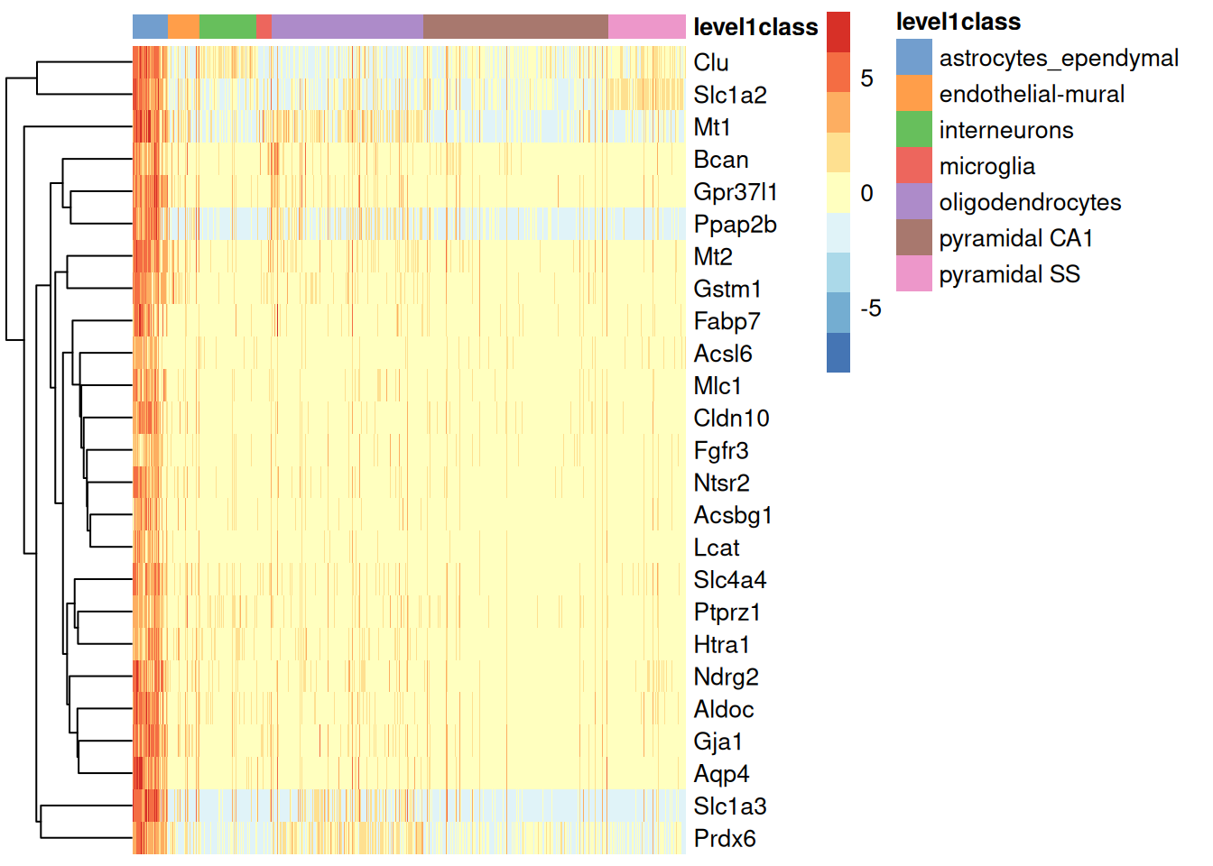
2plotHeatmap( sce.zeisel,
3             features=top.cohen.min,
4             order_columns_by="level1class",
5             center=TRUE
6           )
1plotGroupedHeatmap( sce.zeisel,
2                    features=top.cohen.min,
3                    group="level1class",
4                    center=TRUE
5                  )
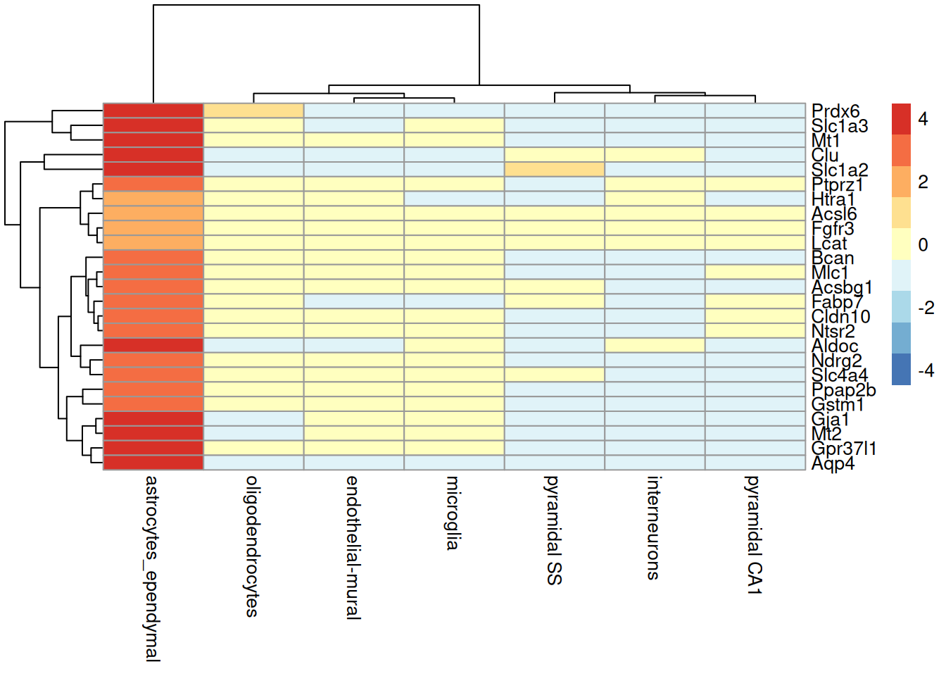
This list is the cleanest of the four, essentially every gene is a canonical, well-established astrocyte marker, with no ambiguous or unusual entries to flag:
- Clu, Gja1, Gpr37l1, Aqp4, Slc1a3, Slc1a2, Aldoc, Cldn10, Ntsr2, Mt2, Ptprz1, Ndrg2, Slc4a4, Mt1, Ppap2b, Bcan, Prdx6, Gstm1: all repeatedly validated astrocyte-enriched genes, same core set seen across the other three lists
- Mlc1, Fabp7 (BLBP), Htra1, Fgfr3, Acsbg1,
Acsl6, Lcat: the same "exclusive/uniquely separating" genes
that were distinctive to
findMarkers.all, reflecting the shared underlying logic of both approaches (see comparison below)
No genes here required flagging. This ranking criterion (minimum Cohen's d across all pairwise comparisons) produced the most conservative and biologically clean marker set of the four.
compare results
 1dataset <- "Zeisel"
 2namedGenesList <- list( findMarkers.all = top.markers, findMarkers.some = top.markers.some,
 3  cohen.median = top.cohen.markers, cohen.min = top.cohen.min
 4)
 5venn.diagram( namedGenesList,
 6                  paste0(dataset, "Venn.diagram.tiff"),
 7                  fill=wes_palette("FantasticFox1")[1:length(namedGenesList)],
 8                  alpha=rep( 0.25, length(namedGenesList) ),
 9                  cex = 2.5, cat.fontface=4,
10                  category.names = names(namedGenesList),
11                  col=wes_palette("FantasticFox1")[1:length(namedGenesList)]
12                )
1## [1] 1
1log.files <- list.files('.', pattern = "*Venn.diagram.*.log", full.names = T)
2file.remove(log.files)
1## [1] TRUE
1cmd <- paste0( 'convert ', dataset, 'Venn.diagram.tiff ', dataset, 'Venn.diagram.png && rm ', dataset, 'Venn.diagram.tiff ' )
2system( cmd )
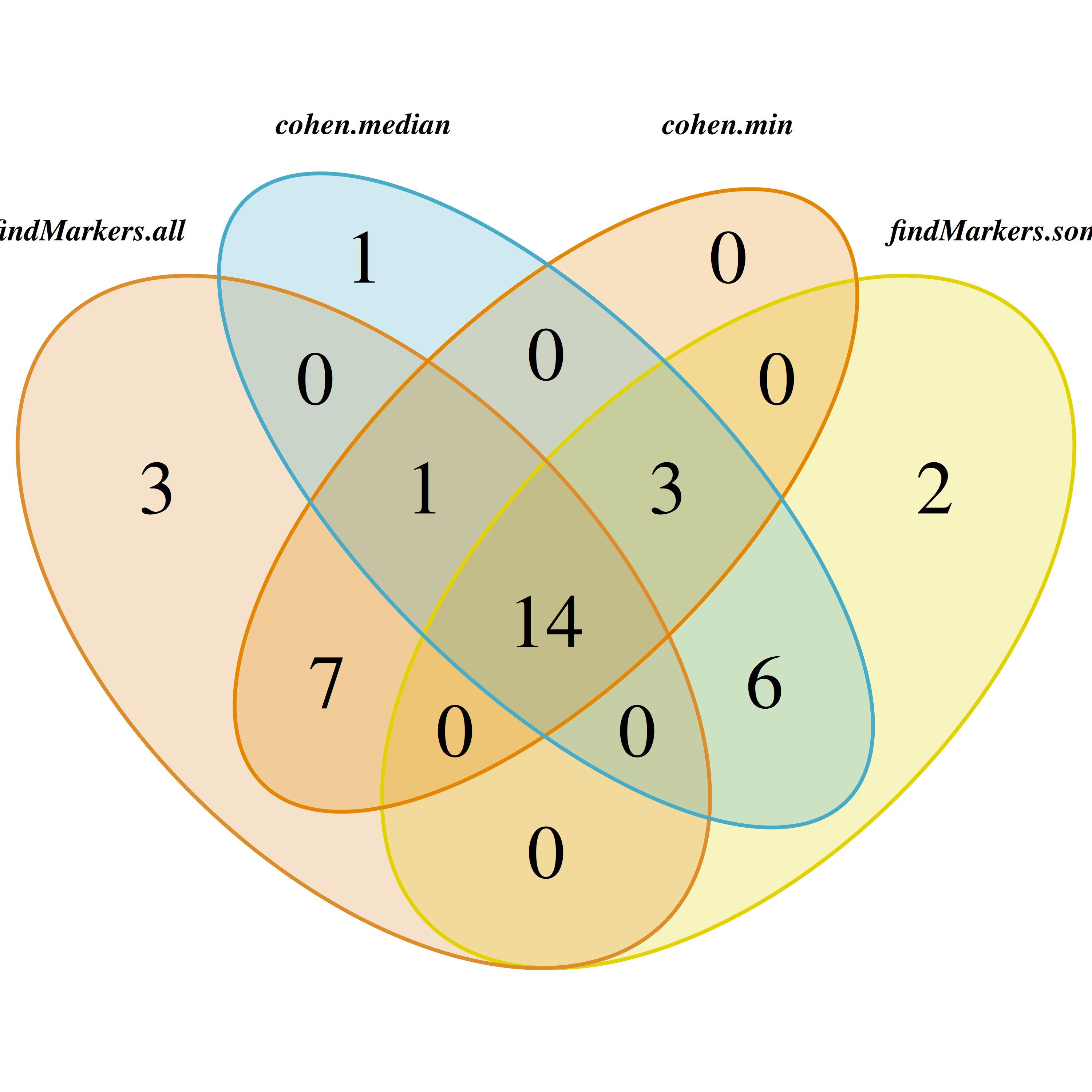
| List | Underlying logic | Character of output | Outlier genes flagged |
|---|---|---|---|
findMarkers.all |
IUT, gene must be DE vs. every other cluster | Clean, exclusive, "uniquely expressed" markers | Scg3, Tmem47 |
findMarkers.some |
Holm-min, gene must be DE vs. most (≥50%) other clusters | Broader, includes top-tier genes missed by all |
Pla2g7, Cst3, Sepp1, Mt1/Mt2 |
cohen.median |
Median effect size across all pairwise comparisons | Very similar composition to findMarkers.some |
Pla2g7, Mmd2, Cst3 |
cohen.min |
Minimum (worst-case) effect size across all pairwise comparisons | Cleanest, most conservative, same logic family as all |
None |
Key pattern: the four lists split into two logic families rather than two methods:
- "Most conservative" logic (
findMarkers.allandcohen.min) both require a gene to hold up against every other cluster, one via a formal intersection-union p-value, the other via the minimum effect size. This shared logic explains whycohen.minrecovers the same "exclusive" genes unique tofindMarkers.all(Mlc1,Fabp7,Htra1,Fgfr3,Acsbg1,Acsl6,Lcat), genes that are strong markers against most, but not necessarily every, cluster equally. - "Majority/average" logic (
findMarkers.someandcohen.median) both reward genes that are DE against most (not all) other clusters, or have a typical (not worst-case) effect size. These two lists converge almost completely (23/25 shared genes) and both surface additional top-tier astrocyte genes (Apoe,Slc1a2,Sparcl1,Atp1a2,Glul) that the stricterall/minapproaches miss, simply because one weak pairwise comparison (e.g. against a very similar glial subtype) is enough to sink them under a worst-case criterion.
Practical takeaway: the "Most conservative" pair (all /
cohen.min) gives the safest, most false-positive-resistant marker set,
ideal for a small validated marker panel. The "majority/average" pair
(some / cohen.median) gives a broader, more sensitive set that
captures more of the true underlying biology (including some of the
most-cited astrocyte genes in the literature) at the cost of
occasionally admitting a less-specific or cross-lineage gene, worth
spot-checking with expression plots before treating as definitive.
Baron pancreas data
- ~8,500–14,000 cells depending on donor, human pancreas
- ~14 annotated cell types (alpha, beta, delta, acinar, ductal, etc.), including some rare populations
1sce.baron <- BaronPancreasData()
check data
1sce.baron
 1## class: SingleCellExperiment
 2## dim: 20125 8569
 3## metadata(0):
 4## assays(1): counts
 5## rownames(20125): A1BG A1CF ... ZZZ3 pk
 6## rowData names(0):
 7## colnames(8569): human1_lib1.final_cell_0001 human1_lib1.final_cell_0002
 8##   ... human4_lib3.final_cell_0700 human4_lib3.final_cell_0701
 9## colData names(2): donor label
10## reducedDimNames(0):
11## mainExpName: NULL
12## altExpNames(0):
The OSCA book does not provide a dedicated Baron pancreas chapter, but we can adapt the Muraro chapter, which is the closest template, since it's also a droplet/CEL-seq-style pancreas dataset with pre-existing cell type labels.
1sce.baron <- addPerCellQC(sce.baron)
2qc <- quickPerCellQC(sce.baron)
3sce.baron <- sce.baron[, !qc$discard]
4sce.baron <- logNormCounts(sce.baron)
5dec <- modelGeneVar(sce.baron)
6top.hvgs <- getTopHVGs(dec, n = 2000)
7sce.baron <- runPCA(sce.baron, subset_row = top.hvgs)
8sce.baron <- runTSNE(sce.baron, dimred = "PCA")
9sce.baron <- runUMAP(sce.baron, dimred = "PCA")
1plotTSNE( sce.baron, colour_by = 'label' )
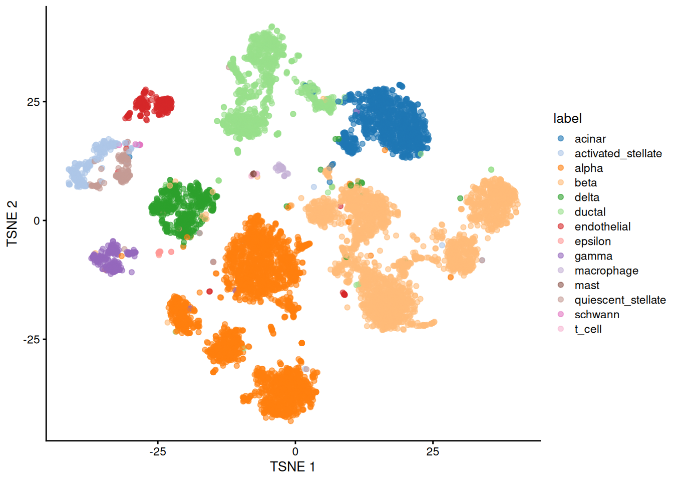
Since the dataset has 4 donors
1table(sce.baron$donor)
1##
2## GSM2230757 GSM2230758 GSM2230759 GSM2230760
3##       1937       1724       3605       1303
we will subset to the donor with highest number of cells
 1sce.baron <- sce.baron[, sce.baron$donor == 'GSM2230759' ]
 2sce.baron <- addPerCellQC(sce.baron)
 3qc <- quickPerCellQC(sce.baron)
 4sce.baron <- sce.baron[, !qc$discard]
 5sce.baron <- logNormCounts(sce.baron)
 6dec <- modelGeneVar(sce.baron)
 7top.hvgs <- getTopHVGs(dec, n = 2000)
 8sce.baron <- runPCA(sce.baron, subset_row = top.hvgs)
 9sce.baron <- runTSNE(sce.baron, dimred = "PCA")
10sce.baron <- runUMAP(sce.baron, dimred = "PCA")
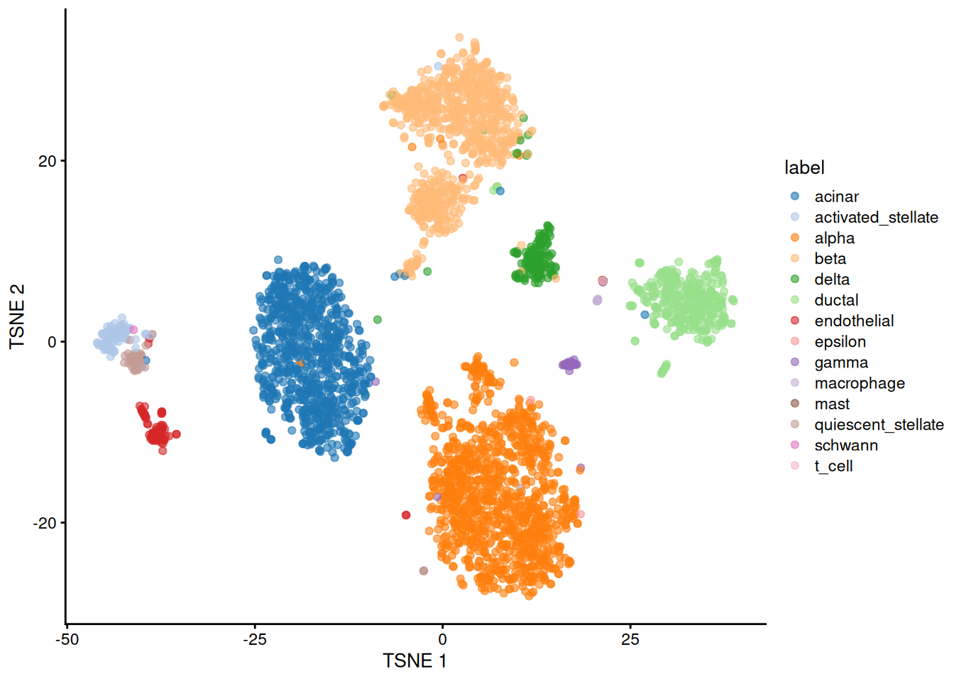
1plotTSNE( sce.baron, colour_by = 'label' )
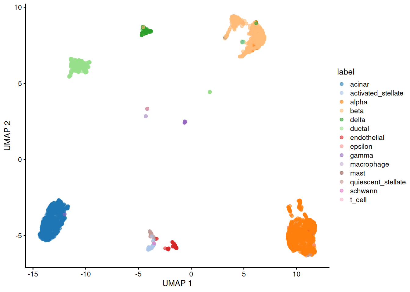
1plotUMAP( sce.baron, colour_by = 'label' )
P-value
all
1markers <- findMarkers( sce.baron, groups = sce.baron$label, direction="up", pval.type = 'all' )
1## Warning in FUN(...): no within-block comparison between schwann and acinar
1## Warning in FUN(...): no within-block comparison between schwann and
2## activated_stellate
1## Warning in FUN(...): no within-block comparison between schwann and alpha
1## Warning in FUN(...): no within-block comparison between schwann and beta
1## Warning in FUN(...): no within-block comparison between schwann and delta
1## Warning in FUN(...): no within-block comparison between schwann and ductal
1## Warning in FUN(...): no within-block comparison between schwann and endothelial
1## Warning in FUN(...): no within-block comparison between schwann and epsilon
1## Warning in FUN(...): no within-block comparison between schwann and gamma
1## Warning in FUN(...): no within-block comparison between schwann and macrophage
1## Warning in FUN(...): no within-block comparison between schwann and mast
1## Warning in FUN(...): no within-block comparison between schwann and
2## quiescent_stellate
1## Warning in FUN(...): no within-block comparison between t_cell and schwann
1names(markers)
1##  [1] "acinar"             "activated_stellate" "alpha"
2##  [4] "beta"               "delta"              "ductal"
3##  [7] "endothelial"        "epsilon"            "gamma"
4## [10] "macrophage"         "mast"               "quiescent_stellate"
5## [13] "schwann"            "t_cell"
We will use Beta cells, a cell type with plently of cells in this dataset and very well-defined markers (INS, insulin)
1marker.set <- markers[["beta"]]
2head(marker.set)
 1## DataFrame with 6 rows and 16 columns
 2##              p.value         FDR summary.logFC logFC.acinar
 3##            <numeric>   <numeric>     <numeric>    <numeric>
 4## ADCYAP1  3.82197e-52 7.69171e-48      2.804818     2.947574
 5## DLK1     7.09409e-51 7.13843e-47      1.165101     1.185885
 6## ENDOD1   3.12929e-31 2.09923e-27      0.599409     0.661405
 7## HADH     4.02317e-27 2.02416e-23      0.903507     1.472314
 8## C1orf127 8.02899e-26 3.23167e-22      0.300417     0.327315
 9## SYNGR4   6.49800e-24 2.17954e-20      1.088293     1.212451
10##          logFC.activated_stellate logFC.alpha logFC.delta logFC.ductal
11##                         <numeric>   <numeric>   <numeric>    <numeric>
12## ADCYAP1                  2.924677    2.907981    2.864506     2.878854
13## DLK1                     1.191400    1.183111    1.159609     1.123609
14## ENDOD1                   0.613597    0.601804    0.632186     0.641972
15## HADH                     1.326232    1.531510    0.903507     1.427523
16## C1orf127                 0.309279    0.316580    0.300417     0.318895
17## SYNGR4                   1.202426    0.537712    1.090644     1.178889
18##          logFC.endothelial logFC.epsilon logFC.gamma logFC.macrophage
19##                  <numeric>     <numeric>   <numeric>        <numeric>
20## ADCYAP1           2.869060      2.978076    2.804818         2.978076
21## DLK1              1.179136      1.203797    1.203797         1.203797
22## ENDOD1            0.599409      0.683211    0.683211         0.683211
23## HADH              1.440996      1.575161    1.575161         1.575161
24## C1orf127          0.332038      0.332038    0.332038         0.332038
25## SYNGR4            1.175324      1.221243    1.188864         1.221243
26##          logFC.mast logFC.quiescent_stellate logFC.schwann logFC.t_cell
27##           <numeric>                <numeric>     <numeric>    <numeric>
28## ADCYAP1    2.978076                 2.859069            NA     2.978076
29## DLK1       1.203797                 1.165101            NA     1.203797
30## ENDOD1     0.683211                 0.657396            NA     0.683211
31## HADH       1.575161                 1.452821            NA     1.575161
32## C1orf127   0.332038                 0.316126            NA     0.332038
33## SYNGR4     1.221243                 1.088293            NA     1.221243
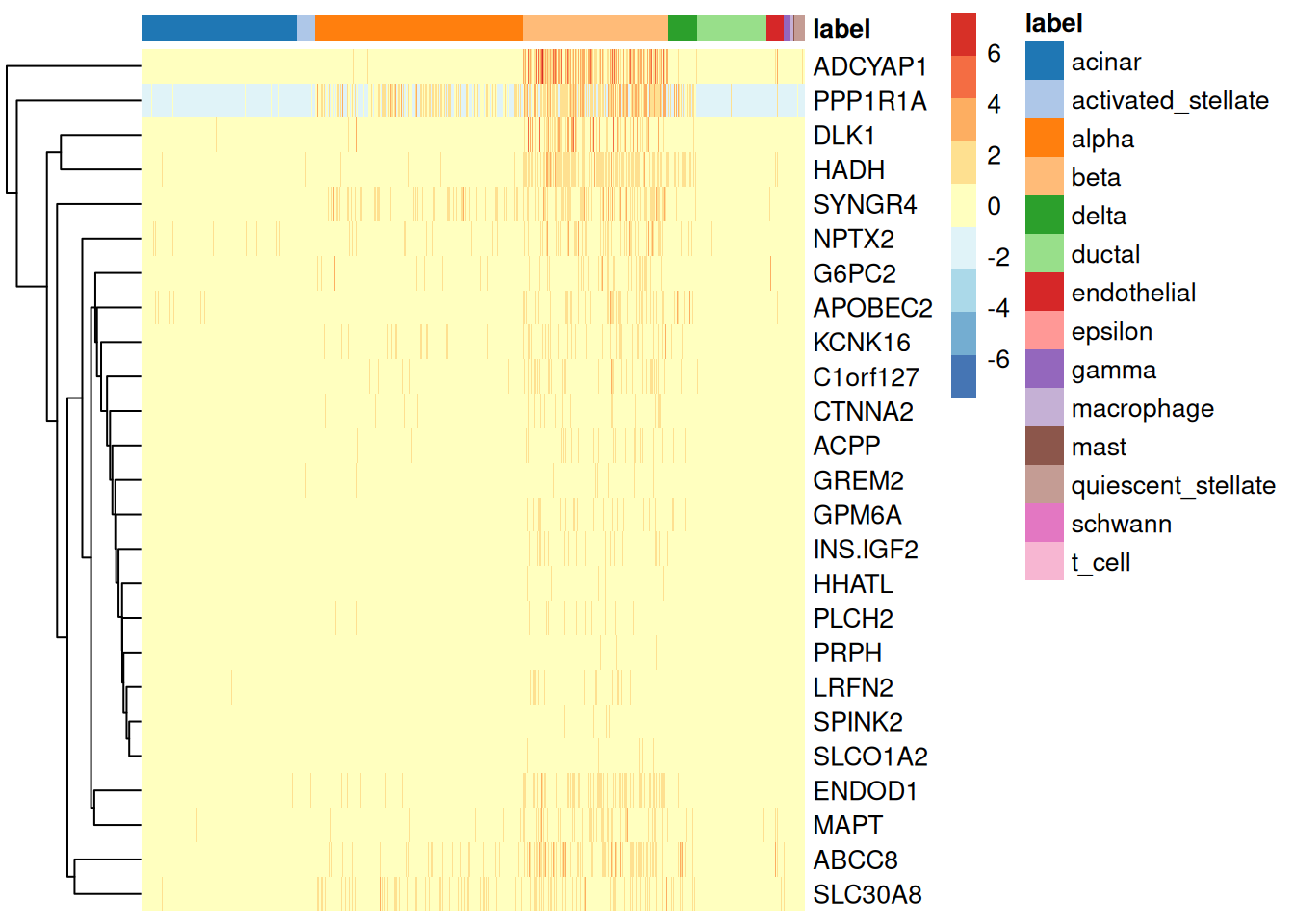
1top.markers <- rownames(marker.set)[1:25]
2plotHeatmap( sce.baron,
3             features=top.markers,
4             order_columns_by="label",
5             center=TRUE
6           )
1plotGroupedHeatmap( sce.baron,
2                    features=top.markers,
3                    group="label",
4                    center=TRUE
5                  )
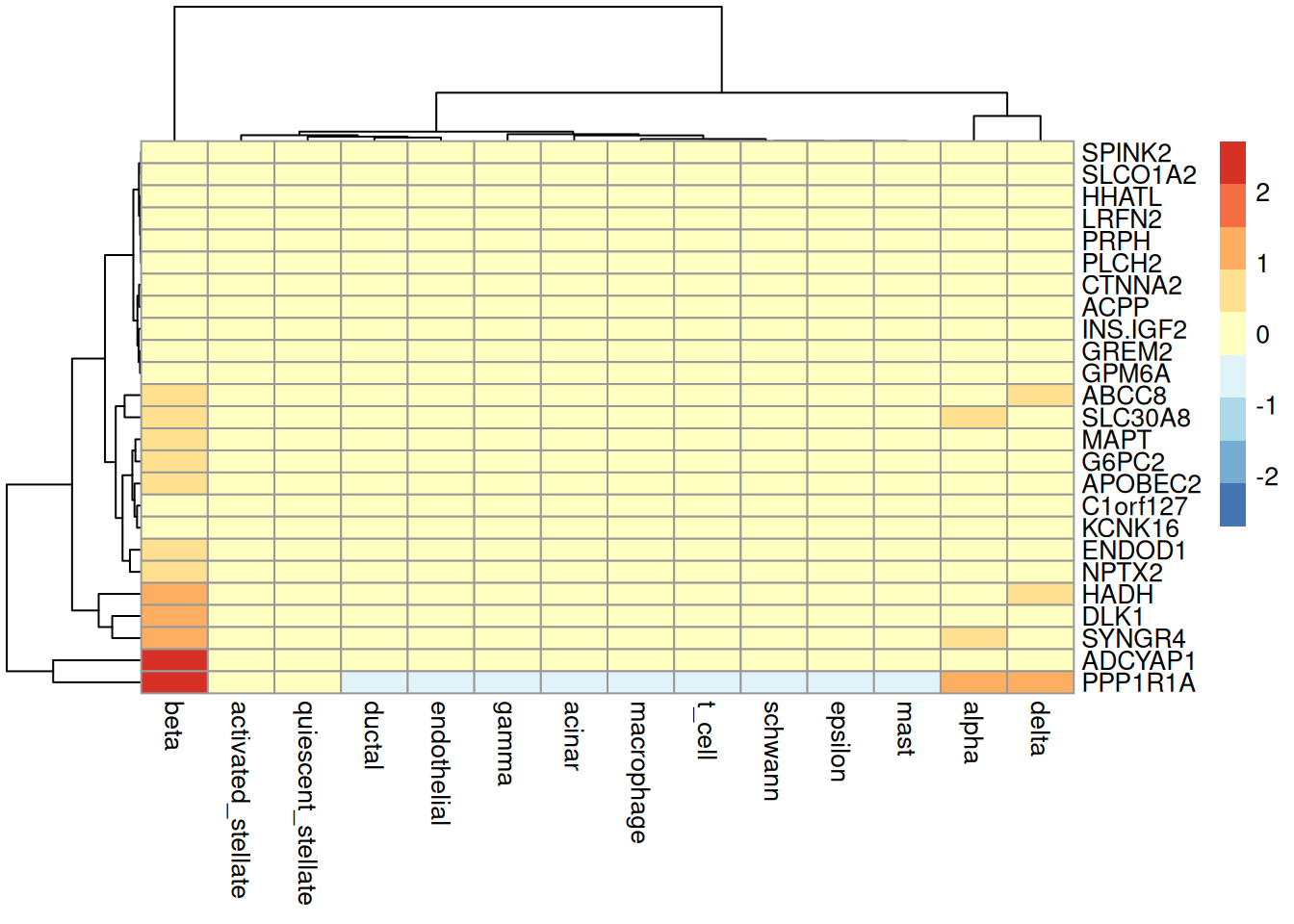
Most are strong, plausible beta-cell markers, several matching known canonical beta-cell biology:
- INS.IGF2: the insulin/IGF2 locus region, essentially the insulin signal itself, the single most definitive beta-cell marker
- ABCC8 (SUR1), KCNK16, G6PC2, SLC30A8 (ZnT8): canonical beta-cell ion channel/metabolic genes central to glucose-sensing and insulin secretion machinery
- HADH: metabolic enzyme repeatedly reported as beta-cell-enriched in human islet scRNA-seq atlases (e.g. Segerstolpe et al.)
- ADCYAP1 (PACAP): repeatedly reported as beta-cell-enriched in human islet studies
- C1orf127: reported as a beta-cell-specific locus in human islet transcriptomic studies
- DLK1: reported as enriched in a subset of human beta cells in several islet atlases
- SPINK2, SYNGR4, PRPH, GPM6A, NPTX2, PLCH2, LRFN2, CTNNA2, HHATL, GREM2, PPP1R1A: plausible beta-cell-enriched genes reported in various human islet single-cell studies, though less "textbook" than the ion-channel/metabolic genes above
Worth a second look:
- MAPT (Tau): more classically a neuronal cytoskeletal gene; its appearance here is plausible given beta cells' neuroendocrine character, but it's not a classic beta marker
- ENDOD1, SLCO1A2, APOBEC2, ACPP: less characterized in beta-cell literature; recommend a sanity check with expression plots
some
1markers <- findMarkers( sce.baron, groups = sce.baron$label, direction="up", pval.type = 'some' )
1## Warning in FUN(...): no within-block comparison between schwann and acinar
1## Warning in FUN(...): no within-block comparison between schwann and
2## activated_stellate
1## Warning in FUN(...): no within-block comparison between schwann and alpha
1## Warning in FUN(...): no within-block comparison between schwann and beta
1## Warning in FUN(...): no within-block comparison between schwann and delta
1## Warning in FUN(...): no within-block comparison between schwann and ductal
1## Warning in FUN(...): no within-block comparison between schwann and endothelial
1## Warning in FUN(...): no within-block comparison between schwann and epsilon
1## Warning in FUN(...): no within-block comparison between schwann and gamma
1## Warning in FUN(...): no within-block comparison between schwann and macrophage
1## Warning in FUN(...): no within-block comparison between schwann and mast
1## Warning in FUN(...): no within-block comparison between schwann and
2## quiescent_stellate
1## Warning in FUN(...): no within-block comparison between t_cell and schwann
1names(markers)
1##  [1] "acinar"             "activated_stellate" "alpha"
2##  [4] "beta"               "delta"              "ductal"
3##  [7] "endothelial"        "epsilon"            "gamma"
4## [10] "macrophage"         "mast"               "quiescent_stellate"
5## [13] "schwann"            "t_cell"
1marker.set <- markers[["beta"]]
2head(marker.set)
 1## DataFrame with 6 rows and 16 columns
 2##              p.value          FDR summary.logFC logFC.acinar
 3##            <numeric>    <numeric>     <numeric>    <numeric>
 4## PPP1R1A 2.10143e-275 4.22912e-271       2.61068      2.61068
 5## NLRP1   1.13034e-250 1.13741e-246       2.03041      2.10552
 6## ADCYAP1 5.53611e-216 3.71381e-212       2.90798      2.94757
 7## HADH    1.52578e-197 7.67658e-194       1.53151      1.47231
 8## PCSK1   3.31573e-133 1.33458e-129       1.23063      1.35322
 9## PCP4    7.66596e-125 2.57129e-121       1.10613      1.13139
10##         logFC.activated_stellate logFC.alpha logFC.delta logFC.ductal
11##                        <numeric>   <numeric>   <numeric>    <numeric>
12## PPP1R1A                  2.50328    1.081112    1.201034      2.51503
13## NLRP1                    1.94944    0.392301   -0.482129      2.03041
14## ADCYAP1                  2.92468    2.907981    2.864506      2.87885
15## HADH                     1.32623    1.531510    0.903507      1.42752
16## PCSK1                    1.29893    1.230633   -0.594472      1.33812
17## PCP4                     1.10460    0.737415   -0.740737      1.10613
18##         logFC.endothelial logFC.epsilon logFC.gamma logFC.macrophage logFC.mast
19##                 <numeric>     <numeric>   <numeric>        <numeric>  <numeric>
20## PPP1R1A           2.57604     2.6480664    2.648066          2.64807    2.64807
21## NLRP1             2.00262     2.1298050    0.509874          2.12980    2.12980
22## ADCYAP1           2.86906     2.9780757    2.804818          2.97808    2.97808
23## HADH              1.44100     1.5751614    1.575161          1.57516    1.57516
24## PCSK1             1.29129    -0.0759007    0.534346          1.36476    1.36476
25## PCP4              1.07768     0.3159199    1.084762          1.13733    1.13733
26##         logFC.quiescent_stellate logFC.schwann logFC.t_cell
27##                        <numeric>     <numeric>    <numeric>
28## PPP1R1A                  2.46717            NA      2.64807
29## NLRP1                    1.82306            NA      2.12980
30## ADCYAP1                  2.85907            NA      2.97808
31## HADH                     1.45282            NA      1.57516
32## PCSK1                    1.30591            NA      1.36476
33## PCP4                     1.13733            NA      1.13733
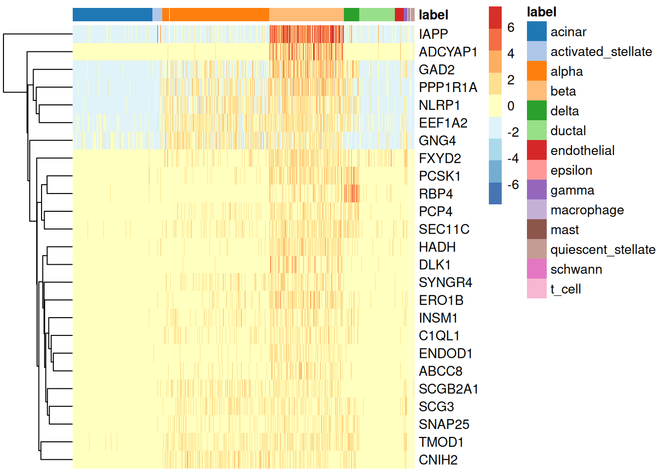
1top.markers.some <- rownames(marker.set)[1:25]
2plotHeatmap( sce.baron,
3             features=top.markers.some,
4             order_columns_by="label",
5             center=TRUE
6           )
1plotGroupedHeatmap( sce.baron,
2                    features=top.markers.some,
3                    group="label",
4                    center=TRUE
5                  )
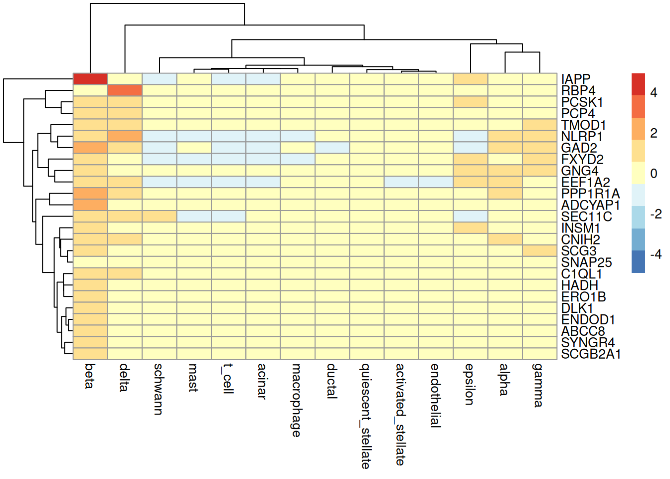
Also strong, with substantial overlap with findMarkers.all, plus several additional
canonical secretory/endocrine genes:
- IAPP (amylin): co-secreted with insulin, one of the most canonical beta-cell markers
, notably absent from
findMarkers.allbut recovered here - PCSK1: proinsulin-processing enzyme, canonical beta-cell secretory machinery gene
- INSM1: pan-endocrine transcription factor, well-established islet marker
- GAD2 (GAD65): in human islets (unlike rodent), GAD65 is a well-documented beta-cell autoantigen and marker
- SNAP25: vesicle-fusion machinery central to regulated hormone secretion
- ADCYAP1, HADH, PPP1R1A, SYNGR4, ENDOD1, ABCC8, DLK1:
overlapping with the
alllist, same canonical status - FXYD2: ion-transport regulatory subunit reported in beta cells
Worth a second look:
- NLRP1: inflammasome component, unusual for a canonical beta marker; could reflect a genuine stress/inflammatory subpopulation or noise
- SCGB2A1 (secretoglobin): more classically associated with epithelial secretory tissues (mammary, prostate) than islet endocrine cells, flag for a sanity check
- RBP4: retinol-binding protein, more classically a liver/adipose-secreted factor; plausible but non-canonical for beta cells specifically
- PCP4, C1QL1, CNIH2, TMOD1: less-characterized in beta-cell-specific literature, some (PCP4) more associated with other islet cell types (e.g. delta cells) in certain atlases
- SEC11C, EEF1A2, ERO1B: general secretory-pathway/translation genes, plausible given beta cells' high secretory demand but not beta-exclusive
- SCG3: chromogranin-family, pan-endocrine rather than beta-specific
Cohen's D
median
1marker.info <- scoreMarkers( sce.baron, groups = sce.baron$label )
2names(marker.info)
1##  [1] "acinar"             "activated_stellate" "alpha"
2##  [4] "beta"               "delta"              "ductal"
3##  [7] "endothelial"        "epsilon"            "gamma"
4## [10] "macrophage"         "mast"               "quiescent_stellate"
5## [13] "schwann"            "t_cell"
1chosen <- marker.info[["beta"]]
2ordered <- chosen[order(chosen$median.logFC.cohen,decreasing=TRUE),]
3head(ordered)
 1## DataFrame with 6 rows and 19 columns
 2##        self.average other.average self.detected other.detected mean.logFC.cohen
 3##           <numeric>     <numeric>     <numeric>      <numeric>        <numeric>
 4## INS        10.30467       2.23340      1.000000       0.747760          5.69385
 5## PCSK1N      3.78043       1.44517      0.993647       0.352881          3.15496
 6## SCG5        3.36036       1.09667      0.974587       0.371592          2.81317
 7## IAPP        5.76456       0.44600      0.954257       0.249669          3.22748
 8## CPE         3.94977       1.34238      0.978399       0.411526          2.65009
 9## GNAS        5.15825       2.69687      0.996188       0.907319          2.45593
10##        min.logFC.cohen median.logFC.cohen max.logFC.cohen rank.logFC.cohen
11##              <numeric>          <numeric>       <numeric>        <integer>
12## INS           3.922247            5.57851         8.52054                1
13## PCSK1N       -1.395328            4.08598         6.72972                1
14## SCG5         -0.591512            3.56926         5.24534                2
15## IAPP          2.673148            3.28697         3.82606                2
16## CPE           0.207575            3.09983         5.18685                3
17## GNAS          0.383697            2.79430         4.52860                3
18##         mean.AUC   min.AUC median.AUC   max.AUC  rank.AUC mean.logFC.detected
19##        <numeric> <numeric>  <numeric> <numeric> <integer>           <numeric>
20## INS     0.995418  0.987641   0.996124  1.000000         1            0.339909
21## PCSK1N  0.775174  0.127700   0.978564  0.996823         1            1.844320
22## SCG5    0.851958  0.300375   0.971840  0.987294         3            1.682381
23## IAPP    0.962887  0.942186   0.964938  0.977128         2            1.706809
24## CPE     0.864538  0.582184   0.972500  0.989199         3            1.450672
25## GNAS    0.926215  0.611872   0.980423  0.993837         2            0.136635
26##        min.logFC.detected median.logFC.detected max.logFC.detected
27##                 <numeric>             <numeric>          <numeric>
28## INS            0.00000000             0.3103401           1.000000
29## PCSK1N        -0.00663086             2.5616449           3.756186
30## SCG5          -0.02465152             1.5603110           3.917464
31## IAPP          -0.04468058             1.8439430           2.382529
32## CPE           -0.03064459             1.3875083           3.733905
33## GNAS          -0.00536079             0.0731451           0.442317
34##        rank.logFC.detected
35##                  <integer>
36## INS                      1
37## PCSK1N                   1
38## SCG5                     3
39## IAPP                     4
40## CPE                      2
41## GNAS                  5020
1top.cohen.markers <- rownames(ordered)[1:length(top.markers)]
2plotHeatmap( sce.baron,
3             features=top.cohen.markers,
4             order_columns_by="label",
5             center=TRUE
6           )
1plotGroupedHeatmap( sce.baron,
2                    features=top.cohen.markers,
3                    group="label",
4                    center=TRUE
5                  )
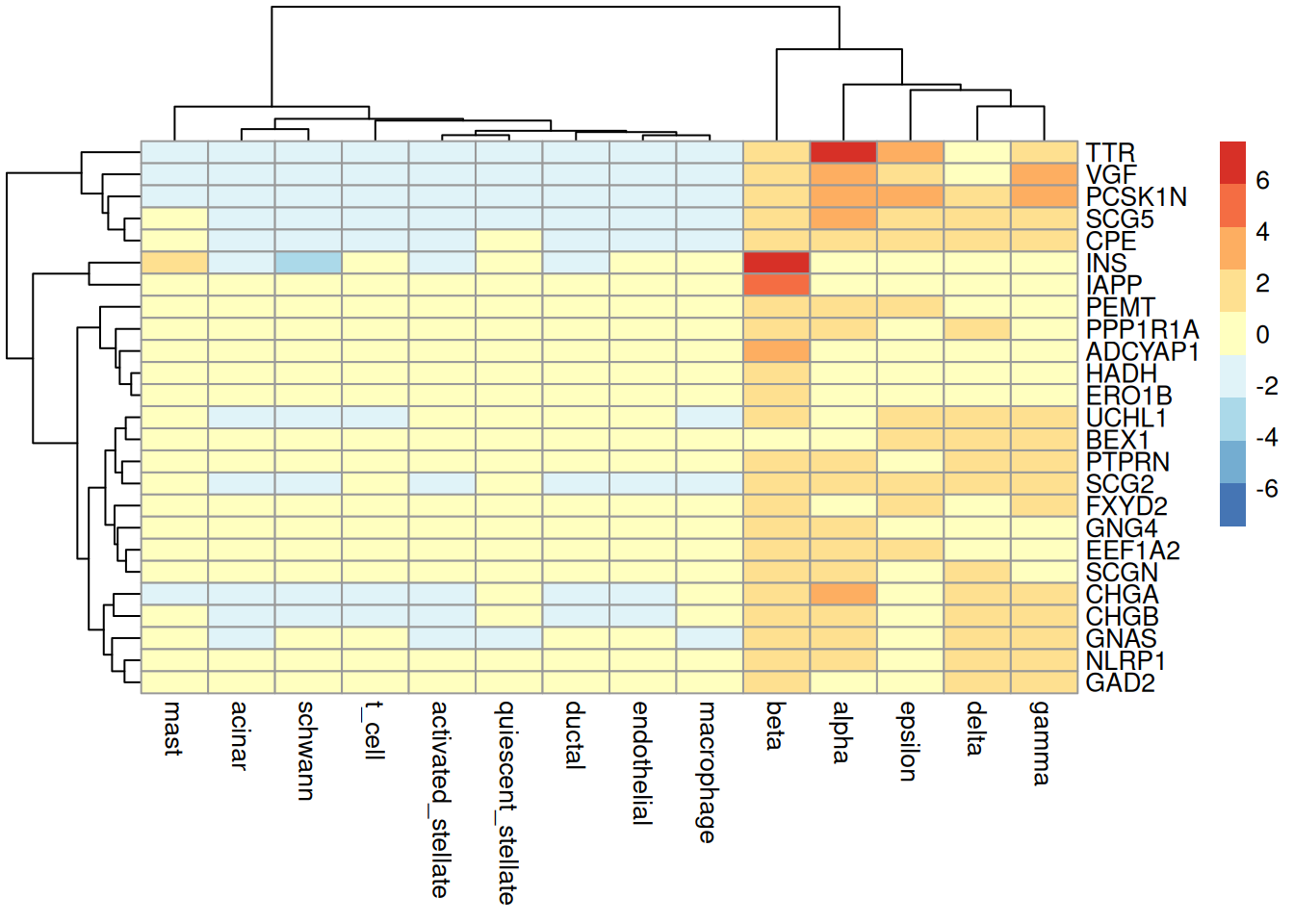
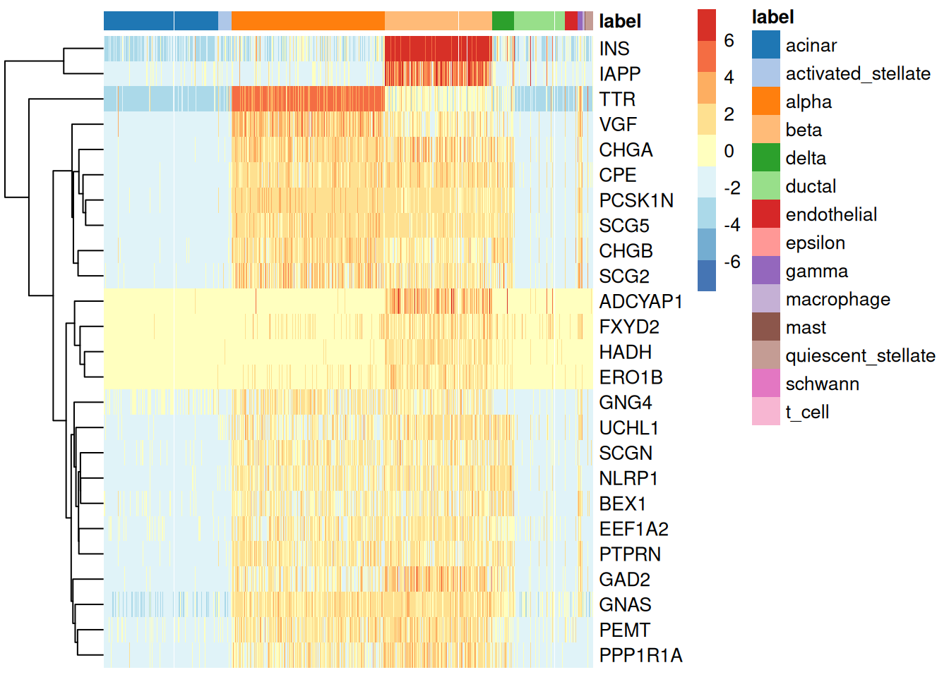
The strongest, most canonical list of the four, dominated by textbook beta-cell identity genes:
- INS: insulin itself, the definitive beta-cell marker, correctly ranked #1
- IAPP, PCSK1N, SCG5, CPE, PTPRN (IA-2), CHGA, CHGB, SCG2, VGF: canonical insulin-processing and secretory-granule genes central to beta-cell identity
- SCGN (secretagogin): well-established islet/beta-cell calcium-binding protein marker
- GNAS, ADCYAP1, HADH, PPP1R1A, GAD2: overlapping with the
findMarkerslists, same canonical status - UCHL1 (PGP9.5): classic neuroendocrine marker, consistent with beta-cell identity
Worth a second look:
- PEMT: phospholipid metabolism enzyme; some literature association with beta cells, but less textbook
- EEF1A2, FXYD2, BEX1: same as before, plausible but not beta-exclusive
- TTR (transthyretin): notable outlier, in several human islet atlases TTR is reported as more alpha- or delta-cell-enriched rather than beta-specific; worth a direct expression check
- GNG4: G-protein subunit, plausible neuroendocrine-secretory association but not classic
min
1ordered <- chosen[order(chosen$min.logFC.cohen,decreasing=TRUE),]
2head(ordered)
 1## DataFrame with 6 rows and 19 columns
 2##         self.average other.average self.detected other.detected
 3##            <numeric>     <numeric>     <numeric>      <numeric>
 4## INS        10.304669     2.2334012      1.000000      0.7477599
 5## IAPP        5.764555     0.4459999      0.954257      0.2496686
 6## ADCYAP1     2.978076     0.0590821      0.871665      0.0319387
 7## DLK1        1.203797     0.0183638      0.459975      0.0108082
 8## ENDOD1      0.683211     0.0288237      0.477764      0.0241528
 9## HADH        1.575161     0.1131713      0.773825      0.0834194
10##         mean.logFC.cohen min.logFC.cohen median.logFC.cohen max.logFC.cohen
11##                <numeric>       <numeric>          <numeric>       <numeric>
12## INS              5.69385        3.922247            5.57851         8.52054
13## IAPP             3.22748        2.673148            3.28697         3.82606
14## ADCYAP1          2.18174        2.059576            2.19313         2.27847
15## DLK1             1.10189        1.013443            1.10931         1.12984
16## ENDOD1           1.13472        0.988859            1.15631         1.22311
17## HADH             1.86643        0.953038            1.95827         2.11988
18##         rank.logFC.cohen  mean.AUC   min.AUC median.AUC   max.AUC  rank.AUC
19##                <integer> <numeric> <numeric>  <numeric> <numeric> <integer>
20## INS                    1  0.995418  0.987641   0.996124  1.000000         1
21## IAPP                   2  0.962887  0.942186   0.964938  0.977128         2
22## ADCYAP1                3  0.928407  0.917902   0.929269  0.935832         3
23## DLK1                  12  0.725817  0.712742   0.726728  0.729987        22
24## ENDOD1                13  0.728405  0.708614   0.729434  0.738882        26
25## HADH                   4  0.863378  0.742386   0.878122  0.886912         4
26##         mean.logFC.detected min.logFC.detected median.logFC.detected
27##                   <numeric>          <numeric>             <numeric>
28## INS                0.339909          0.0000000               0.31034
29## IAPP               1.706809         -0.0446806               1.84394
30## ADCYAP1            3.278615          0.9043219               3.75832
31## DLK1               3.161470          0.5459433               3.64493
32## ENDOD1             2.672024          0.5634156               2.94207
33## HADH               2.556059          0.8227821               2.60465
34##         max.logFC.detected rank.logFC.detected
35##                  <numeric>           <integer>
36## INS                1.00000                   1
37## IAPP               2.38253                   4
38## ADCYAP1            4.61303                   4
39## DLK1               4.98694                   4
40## ENDOD1             4.18583                   3
41## HADH               4.85088                   2
1top.cohen.min <- rownames(ordered)[1:length(top.markers)]
2plotHeatmap( sce.baron,
3             features=top.cohen.min,
4             order_columns_by="label",
5             center=TRUE
6           )
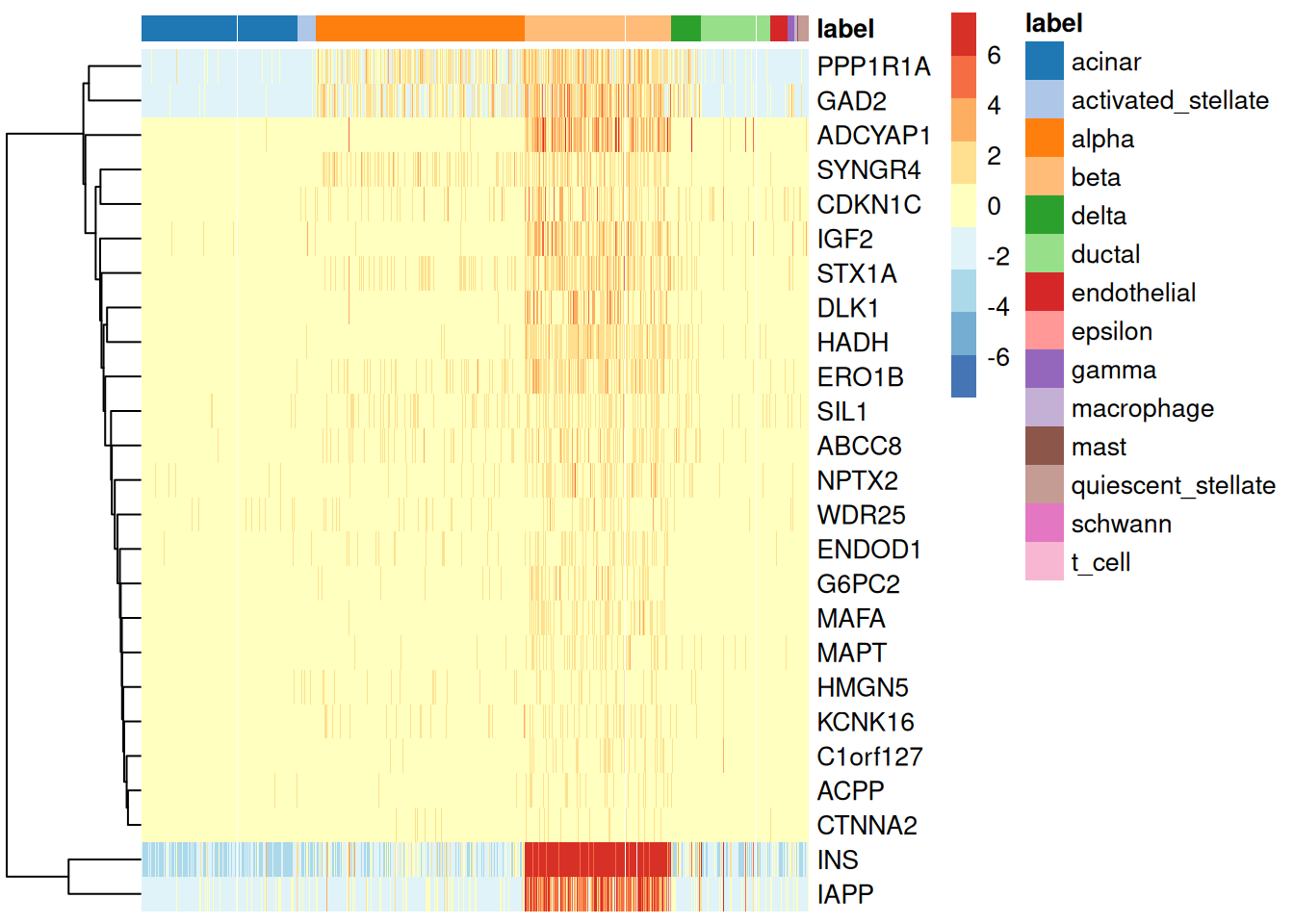
1plotGroupedHeatmap( sce.baron,
2                    features=top.cohen.min,
3                    group="label",
4                    center=TRUE
5                  )
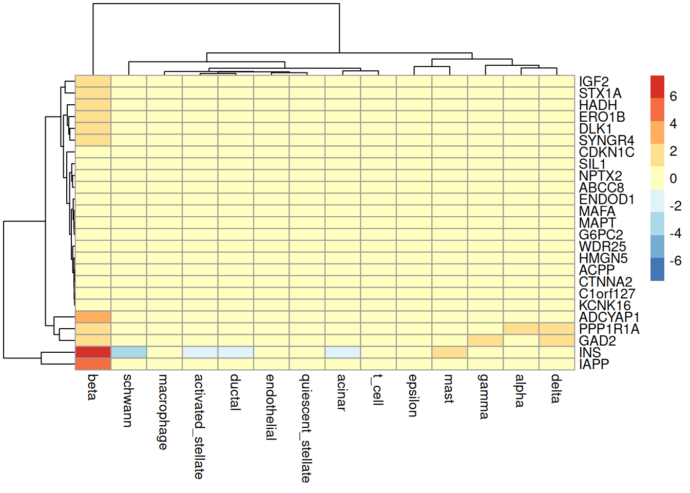
Also very strong, with the same canonical core as findMarkers.all, reinforcing that both "worst-case" criteria converge well here:
- INS, IAPP: correctly recovered, INS at rank #1
- MAFA: canonical beta-cell master transcription factor, a strong addition not seen
in either
findMarkerslist - ABCC8, G6PC2, KCNK16, ADCYAP1, HADH, PPP1R1A, GAD2,
C1orf127, NPTX2, SYNGR4, ACPP, CTNNA2: overlapping with
findMarkers.all, same canonical/plausible status - IGF2: consistent with the
INS.IGF2locus signal seen infindMarkers.all - CDKN1C (p57): reported as enriched in mature, non-proliferating beta cells in several human islet studies
- STX1A: canonical exocytosis-machinery gene central to regulated insulin secretion
- MAPT, ENDOD1, DLK1: same as
findMarkers.all
Worth a second look:
- SIL1, WDR25, HMGN5: less-characterized in beta-cell-specific literature
compare results
 1dataset <- "Baron"
 2namedGenesList <- list( findMarkers.all = top.markers, findMarkers.some = top.markers.some,
 3  cohen.median = top.cohen.markers, cohen.min = top.cohen.min
 4)
 5venn.diagram( namedGenesList,
 6                  paste0(dataset, "Venn.diagram.tiff"),
 7                  fill=wes_palette("FantasticFox1")[1:length(namedGenesList)],
 8                  alpha=rep( 0.25, length(namedGenesList) ),
 9                  cex = 2.5, cat.fontface=4,
10                  category.names = names(namedGenesList),
11                  col=wes_palette("FantasticFox1")[1:length(namedGenesList)]
12                )
1## [1] 1
1log.files <- list.files('.', pattern = "*Venn.diagram.*.log", full.names = T)
2file.remove(log.files)
1## [1] TRUE
1cmd <- paste0( 'convert ', dataset, 'Venn.diagram.tiff ', dataset, 'Venn.diagram.png && rm ', dataset, 'Venn.diagram.tiff ' )
2system( cmd )
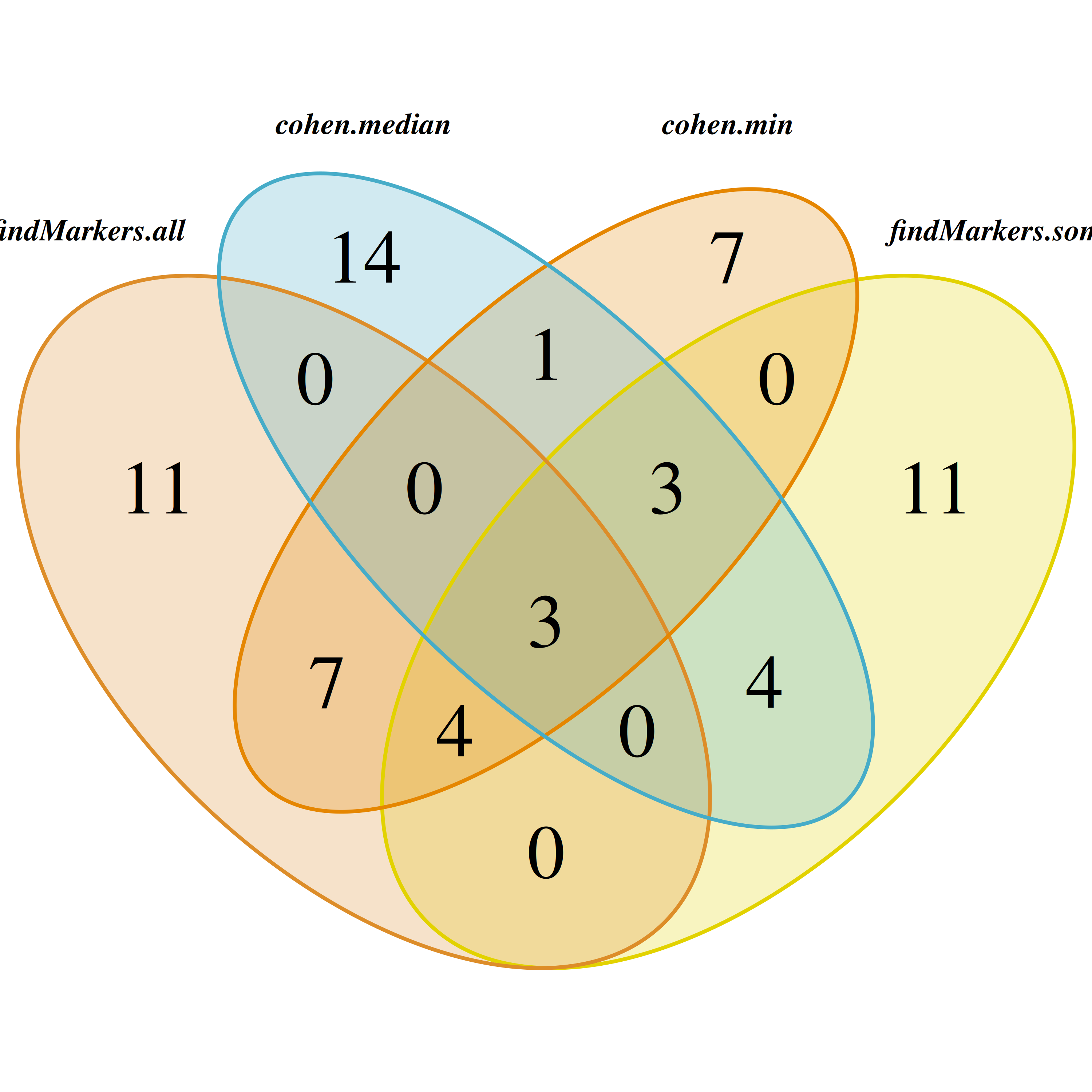
| List | Canonical hits (INS/IAPP/MAFA/etc.) | Overall signal quality | Outlier genes flagged |
|---|---|---|---|
findMarkers.all |
INS.IGF2, ABCC8, G6PC2, SLC30A8, HADH | Strong | MAPT, ENDOD1, SLCO1A2, APOBEC2, ACPP |
findMarkers.some |
IAPP, PCSK1, INSM1, GAD2, SNAP25 | Strong, broader secretory-pathway coverage | NLRP1, SCGB2A1, RBP4, PCP4, C1QL1 |
cohen.median |
INS (#1), IAPP, PTPRN, CHGA, CHGB, SCGN | Strongest — most textbook genes at top ranks | TTR, PEMT, GNG4 |
cohen.min |
INS (#1), IAPP, MAFA, STX1A, CDKN1C | Strongest — best coverage of both hormone and TF/exocytosis machinery | SIL1, WDR25, HMGN5 |
Key contrast with the epsilon cell results: unlike epsilon cells, where findMarkers
badly under-recovered the canonical marker (GHRL absent from "some", buried at rank 14 in
"all") and only scoreMarkers reliably found it, all four methods correctly rank INS
(or the INS-linked locus) at or near the top for beta cells, and all four surface a
substantial, overlapping core of well-established beta-cell genes (IAPP, ABCC8, HADH,
ADCYAP1, PPP1R1A, GAD2, G6PC2, C1orf127, DLK1, ENDOD1, SYNGR4).
This is the expected "positive control" behavior: with a large, abundant, transcriptionally
distinct cluster, statistical power is high enough that both p-value-based (findMarkers)
and effect-size-based (scoreMarkers) approaches converge on the same biological answer,
regardless of the specific combining rule (all/some/median/min) used. This
reinforces the interpretation from the epsilon cell case: the divergence between
findMarkers and scoreMarkers is driven primarily by cluster size and effect magnitude,
not by an inherent flaw in either method — with enough cells and a strong enough
biological signal, both methods agree well.
Rare cell type
The previous tests focused on very clear cell types with many cells in the dataset. For stress-testing these methods, we will focus now in Epsilon cells. Epsilon cells (ghrelin-producing) are consistently the smallest endocrine population in pancreatic islet atlases, which makes them an ideal stress test.
P-value
all
1markers <- findMarkers( sce.baron, groups = sce.baron$label, direction="up", pval.type = 'all' )
1## Warning in FUN(...): no within-block comparison between schwann and acinar
1## Warning in FUN(...): no within-block comparison between schwann and
2## activated_stellate
1## Warning in FUN(...): no within-block comparison between schwann and alpha
1## Warning in FUN(...): no within-block comparison between schwann and beta
1## Warning in FUN(...): no within-block comparison between schwann and delta
1## Warning in FUN(...): no within-block comparison between schwann and ductal
1## Warning in FUN(...): no within-block comparison between schwann and endothelial
1## Warning in FUN(...): no within-block comparison between schwann and epsilon
1## Warning in FUN(...): no within-block comparison between schwann and gamma
1## Warning in FUN(...): no within-block comparison between schwann and macrophage
1## Warning in FUN(...): no within-block comparison between schwann and mast
1## Warning in FUN(...): no within-block comparison between schwann and
2## quiescent_stellate
1## Warning in FUN(...): no within-block comparison between t_cell and schwann
1names(markers)
1##  [1] "acinar"             "activated_stellate" "alpha"
2##  [4] "beta"               "delta"              "ductal"
3##  [7] "endothelial"        "epsilon"            "gamma"
4## [10] "macrophage"         "mast"               "quiescent_stellate"
5## [13] "schwann"            "t_cell"
Select Epsilon cells.
1marker.set <- markers[["epsilon"]]
2head(marker.set)
 1## DataFrame with 6 rows and 16 columns
 2##             p.value       FDR summary.logFC logFC.acinar
 3##           <numeric> <numeric>     <numeric>    <numeric>
 4## CLU      0.00162492         1       5.83598      5.10869
 5## C10orf10 0.00291337         1       2.85518      2.54781
 6## DNAJC12  0.00357871         1       2.04196      1.86718
 7## EIF4A1   0.00357871         1       2.04196      1.03643
 8## TMEM59   0.00357871         1       2.04196      1.63054
 9## ITFG1    0.00357890         1       2.04196      1.96372
10##          logFC.activated_stellate logFC.alpha logFC.beta logFC.delta
11##                         <numeric>   <numeric>  <numeric>   <numeric>
12## CLU                       5.19351    0.676458   4.286503    2.868398
13## C10orf10                  2.76758    1.579832   1.177291    2.081857
14## DNAJC12                   1.94468    0.925978   0.585280    0.823184
15## EIF4A1                    0.73903    1.219088   1.546688    1.451831
16## TMEM59                    1.30457    0.687245   0.572086    0.543979
17## ITFG1                     1.89768    1.798522   1.806795    1.809807
18##          logFC.ductal logFC.endothelial logFC.gamma logFC.macrophage logFC.mast
19##             <numeric>         <numeric>   <numeric>        <numeric>  <numeric>
20## CLU          4.424696           5.53682    1.477849          5.74437    1.98222
21## C10orf10     2.362217           2.08370    2.338561          2.85518    2.85518
22## DNAJC12      1.994867           2.00371    0.603961          1.90655    1.76280
23## EIF4A1       0.806659           1.02513    1.515684          1.31952    1.72868
24## TMEM59       1.299768           1.29398    0.847936          1.45605    1.50853
25## ITFG1        1.896463           1.92235    1.711640          1.84485    2.04196
26##          logFC.quiescent_stellate logFC.schwann logFC.t_cell
27##                         <numeric>     <numeric>    <numeric>
28## CLU                      5.325832            NA      5.83598
29## C10orf10                 2.802829            NA      2.85518
30## DNAJC12                  1.882799            NA      2.04196
31## EIF4A1                   0.571178            NA      2.04196
32## TMEM59                   1.285782            NA      2.04196
33## ITFG1                    1.970115            NA      2.04196
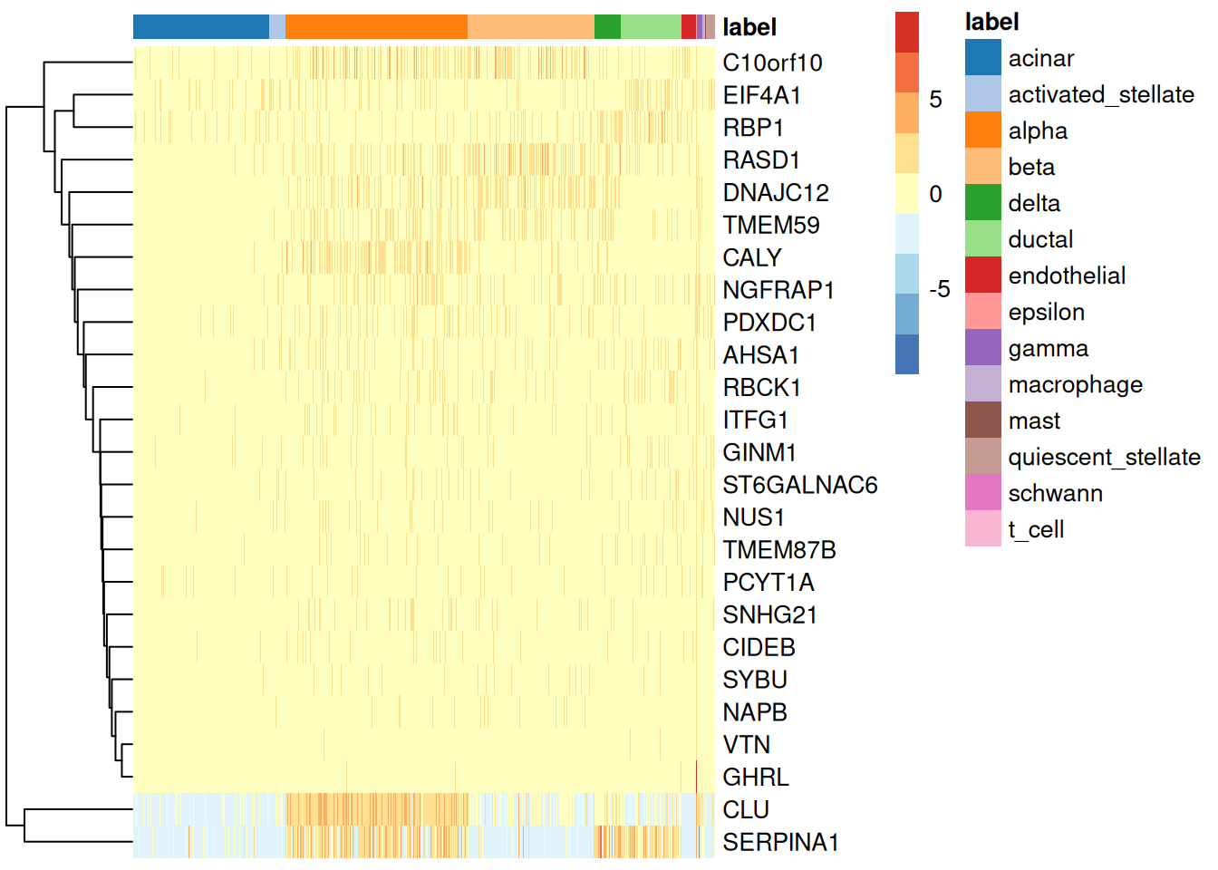
No significant (FDR < 0.05) where found, we will continue with the top genes for comparative purposes.
1top.markers <- rownames(marker.set)[1:25]
2plotHeatmap( sce.baron,
3             features=top.markers,
4             order_columns_by="label",
5             center=TRUE
6           )
1plotGroupedHeatmap( sce.baron,
2                    features=top.markers,
3                    group="label",
4                    center=TRUE
5                  )
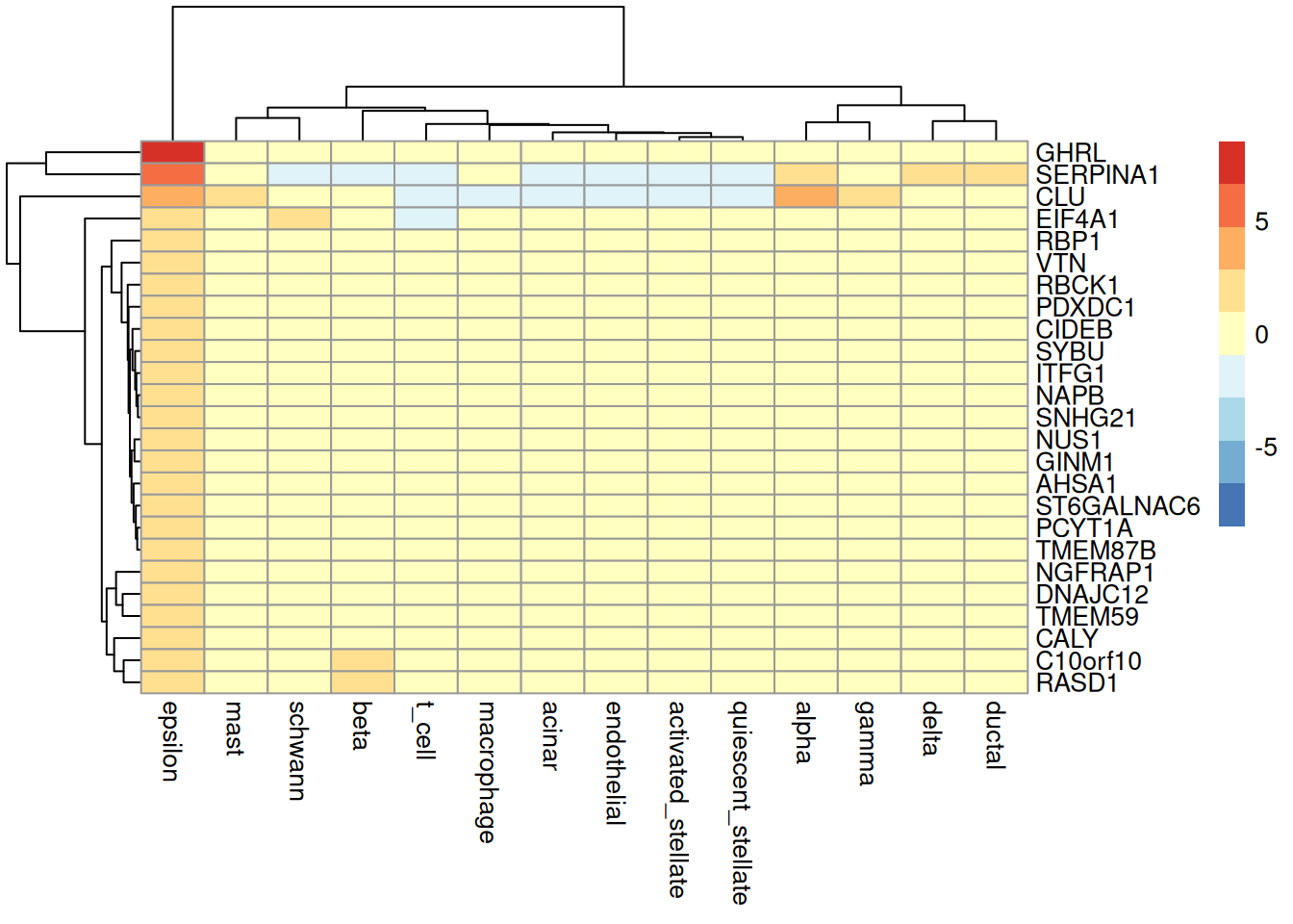
Only a few genes here are epsilon-specific, and even the one unambiguous marker is buried mid-list rather than at the top:
- GHRL: ghrelin, epsilon cells are identified by high GHRL expression, and this is the single most-established epsilon marker in the literature. Its presence at rank 14 (not top-ranked) despite being the canonical, near-exclusive marker for this cell type is itself a signal that a strict "beat every other cluster" p-value criterion loses power with very few cells.
- SERPINA1, VTN: not classic epsilon markers, more associated with liver/exocrine or vascular biology; plausibly reflect ambient RNA contamination given the tiny cluster size
- CLU, RBCK1, DNAJC12, EIF4A1, TMEM59, ITFG1, ST6GALNAC6, RBP1, SYBU, CIDEB, NGFRAP1, CALY, RASD1, AHSA1, PDXDC1, NAPB, PCYT1A, TMEM87B, NUS1, GINM1, SNHG21, C10orf10: largely generic/housekeeping genes (translation factors, ubiquitin-related, lipid metabolism, ribosomal/RNA-processing) without established epsilon-specific biology in the literature, most likely likely statistical noise from testing with so few cells, rather than genuine markers
some
1markers <- findMarkers( sce.baron, groups = sce.baron$label, direction="up", pval.type = 'some' )
1## Warning in FUN(...): no within-block comparison between schwann and acinar
1## Warning in FUN(...): no within-block comparison between schwann and
2## activated_stellate
1## Warning in FUN(...): no within-block comparison between schwann and alpha
1## Warning in FUN(...): no within-block comparison between schwann and beta
1## Warning in FUN(...): no within-block comparison between schwann and delta
1## Warning in FUN(...): no within-block comparison between schwann and ductal
1## Warning in FUN(...): no within-block comparison between schwann and endothelial
1## Warning in FUN(...): no within-block comparison between schwann and epsilon
1## Warning in FUN(...): no within-block comparison between schwann and gamma
1## Warning in FUN(...): no within-block comparison between schwann and macrophage
1## Warning in FUN(...): no within-block comparison between schwann and mast
1## Warning in FUN(...): no within-block comparison between schwann and
2## quiescent_stellate
1## Warning in FUN(...): no within-block comparison between t_cell and schwann
1names(markers)
1##  [1] "acinar"             "activated_stellate" "alpha"
2##  [4] "beta"               "delta"              "ductal"
3##  [7] "endothelial"        "epsilon"            "gamma"
4## [10] "macrophage"         "mast"               "quiescent_stellate"
5## [13] "schwann"            "t_cell"
1marker.set <- markers[["epsilon"]]
2head(marker.set)
 1## DataFrame with 6 rows and 16 columns
 2##              p.value         FDR summary.logFC logFC.acinar
 3##            <numeric>   <numeric>     <numeric>    <numeric>
 4## CLU      1.39031e-17 2.79799e-13      5.744375      5.10869
 5## RBCK1    8.63534e-16 8.68931e-12      1.491910      1.72944
 6## PPP2R1A  8.50449e-15 5.70509e-11      1.837770      2.10601
 7## C10orf10 5.73089e-14 2.88335e-10      2.767581      2.54781
 8## RBP1     7.15700e-13 2.88069e-09      1.494734      1.19092
 9## LRRFIP1  1.00735e-11 3.37883e-08      0.599206      1.46438
10##          logFC.activated_stellate logFC.alpha logFC.beta logFC.delta
11##                         <numeric>   <numeric>  <numeric>   <numeric>
12## CLU                       5.19351    0.676458    4.28650    2.868398
13## RBCK1                     1.89499    1.569998    1.71417    1.799870
14## PPP2R1A                   1.50579    1.585841    1.92267    1.958516
15## C10orf10                  2.76758    1.579832    1.17729    2.081857
16## RBP1                      1.72283    1.647284    1.63449    0.984536
17## LRRFIP1                   1.46639    1.301833    1.82010    1.666693
18##          logFC.ductal logFC.endothelial logFC.gamma logFC.macrophage logFC.mast
19##             <numeric>         <numeric>   <numeric>        <numeric>  <numeric>
20## CLU          4.424696           5.53682     1.47785          5.74437   1.982218
21## RBCK1        1.491910           1.88664     1.84736          1.96061   1.420154
22## PPP2R1A      1.226239           1.77772     1.98399          2.12545   1.853787
23## C10orf10     2.362217           2.08370     2.33856          2.85518   2.855182
24## RBP1         0.817196           1.60877     1.49473          2.04196   2.041960
25## LRRFIP1      0.599206           1.54870     1.62696          1.31015   0.636798
26##          logFC.quiescent_stellate logFC.schwann logFC.t_cell
27##                         <numeric>     <numeric>    <numeric>
28## CLU                       5.32583            NA      5.83598
29## RBCK1                     1.82740            NA      2.04196
30## PPP2R1A                   1.83777            NA      1.43285
31## C10orf10                  2.80283            NA      2.85518
32## RBP1                      1.63215            NA      2.04196
33## LRRFIP1                   1.53628            NA      1.01602
1top.markers.some <- rownames(marker.set)[1:25]
2plotHeatmap( sce.baron,
3             features=top.markers.some,
4             order_columns_by="label",
5             center=TRUE
6           )
1plotGroupedHeatmap( sce.baron,
2                    features=top.markers.some,
3                    group="label",
4                    center=TRUE
5                  )
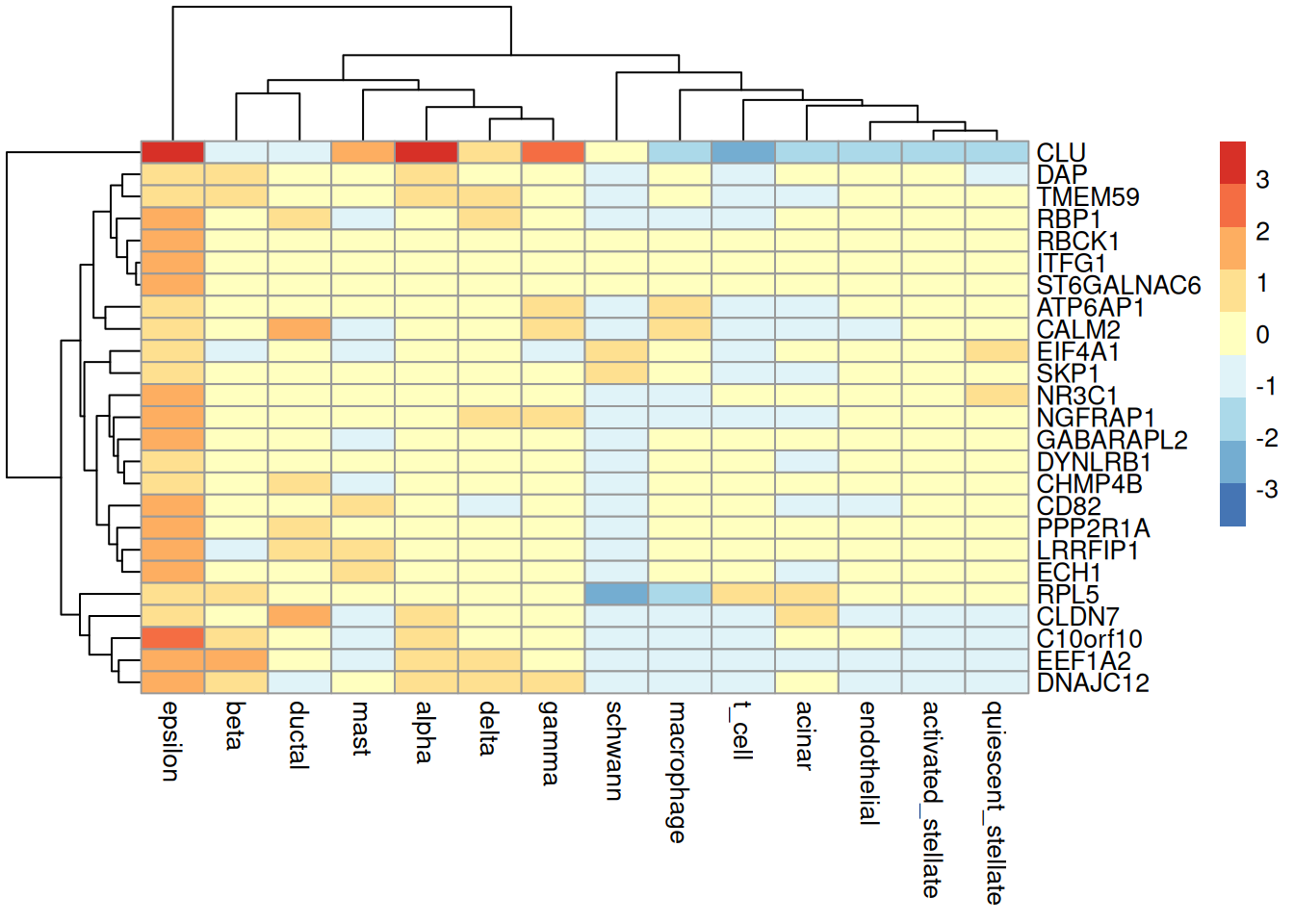
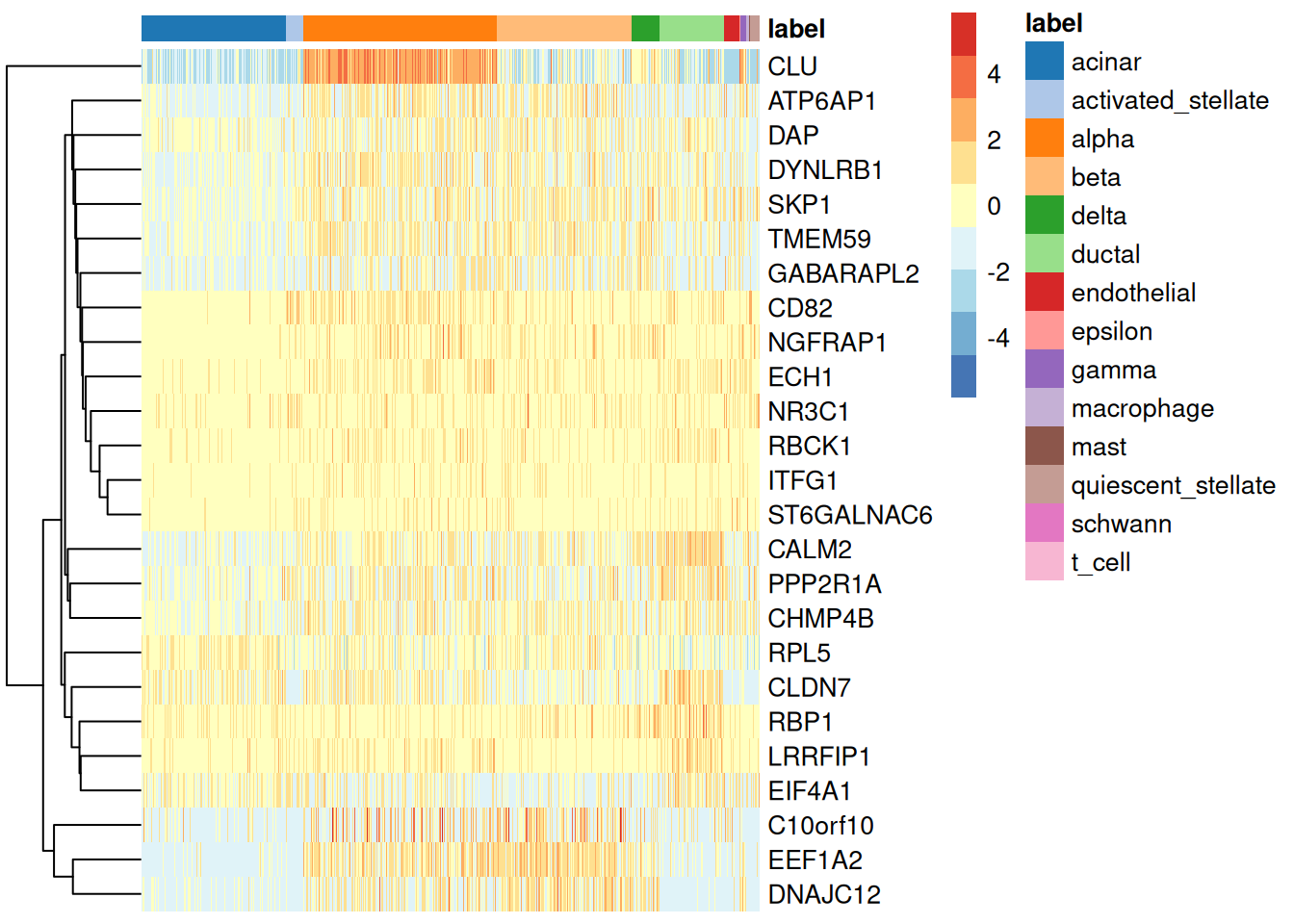
Notably worse: GHRL does not appear anywhere in this top-25 list at all, a real red flag for this parameterization on a rare cell type.
- Nearly the entire list (RPL5, EEF1A2, CALM2, SKP1, ATP6AP1, DYNLRB1, GABARAPL2, CHMP4B, LRRFIP1, ECH1, CD82, DAP, NR3C1, PPP2R1A) consists of broadly-expressed housekeeping/translation/vesicle-trafficking genes with no epsilon-specific role documented
- This is the weakest of the four lists, with
"some"'s majority-vote logic combined with very low cell numbers, the ranking appears to be dominated by noise rather than biology
Cohen's D
median
1marker.info <- scoreMarkers( sce.baron, groups = sce.baron$label )
2names(marker.info)
1##  [1] "acinar"             "activated_stellate" "alpha"
2##  [4] "beta"               "delta"              "ductal"
3##  [7] "endothelial"        "epsilon"            "gamma"
4## [10] "macrophage"         "mast"               "quiescent_stellate"
5## [13] "schwann"            "t_cell"
1chosen <- marker.info[["epsilon"]]
2ordered <- chosen[order(chosen$median.logFC.cohen,decreasing=TRUE),]
3head(ordered)
 1## DataFrame with 6 rows and 19 columns
 2##         self.average other.average self.detected other.detected
 3##            <numeric>     <numeric>     <numeric>      <numeric>
 4## VTN          2.74298    0.00533242             1     0.00497212
 5## GHRL         9.19138    0.00164257             1     0.00131614
 6## SYBU         2.04196    0.03471349             1     0.02799088
 7## CALY         3.21008    0.23398177             1     0.13566012
 8## CIDEB        2.04196    0.08525482             1     0.05109872
 9## TMEM179      1.83091    0.06949539             1     0.05435582
10##         mean.logFC.cohen min.logFC.cohen median.logFC.cohen max.logFC.cohen
11##                <numeric>       <numeric>          <numeric>       <numeric>
12## VTN             28.37347        16.94799           31.87112         31.8711
13## GHRL            24.18584        23.74169           24.29966         24.2997
14## SYBU            38.59628         5.60475           18.56236         88.9349
15## CALY            14.13938         2.33228           16.25252         23.8458
16## CIDEB           28.27451         2.71421           10.29078         88.9349
17## TMEM179          7.67959         3.36127            9.29101          9.7340
18##         rank.logFC.cohen  mean.AUC   min.AUC median.AUC   max.AUC  rank.AUC
19##                <integer> <numeric> <numeric>  <numeric> <numeric> <integer>
20## VTN                    1  1.000000  1.000000          1         1         1
21## GHRL                   1  1.000000  1.000000          1         1         1
22## SYBU                   1  0.998219  0.987929          1         1         1
23## CALY                   3  0.995919  0.951327          1         1         1
24## CIDEB                  1  0.980123  0.857143          1         1         1
25## TMEM179                7  0.994246  0.968584          1         1         1
26##         mean.logFC.detected min.logFC.detected median.logFC.detected
27##                   <numeric>          <numeric>             <numeric>
28## VTN                 1.52593           1.000000               1.58496
29## GHRL                1.53619           1.000000               1.58496
30## SYBU                1.46471           1.000000               1.50696
31## CALY                1.25261           0.435899               1.49381
32## CIDEB               1.40517           1.000000               1.43296
33## TMEM179             1.40462           1.000000               1.56970
34##         max.logFC.detected rank.logFC.detected
35##                  <numeric>           <integer>
36## VTN                1.58496                   1
37## GHRL               1.58496                   1
38## SYBU               1.58496                   1
39## CALY               1.58496                   1
40## CIDEB              1.58496                   1
41## TMEM179            1.58496                   1
1top.cohen.markers <- rownames(ordered)[1:length(top.markers)]
2plotHeatmap( sce.baron,
3             features=top.cohen.markers,
4             order_columns_by="label",
5             center=TRUE
6           )
1plotGroupedHeatmap( sce.baron,
2                    features=top.cohen.markers,
3                    group="label",
4                    center=TRUE
5                  )
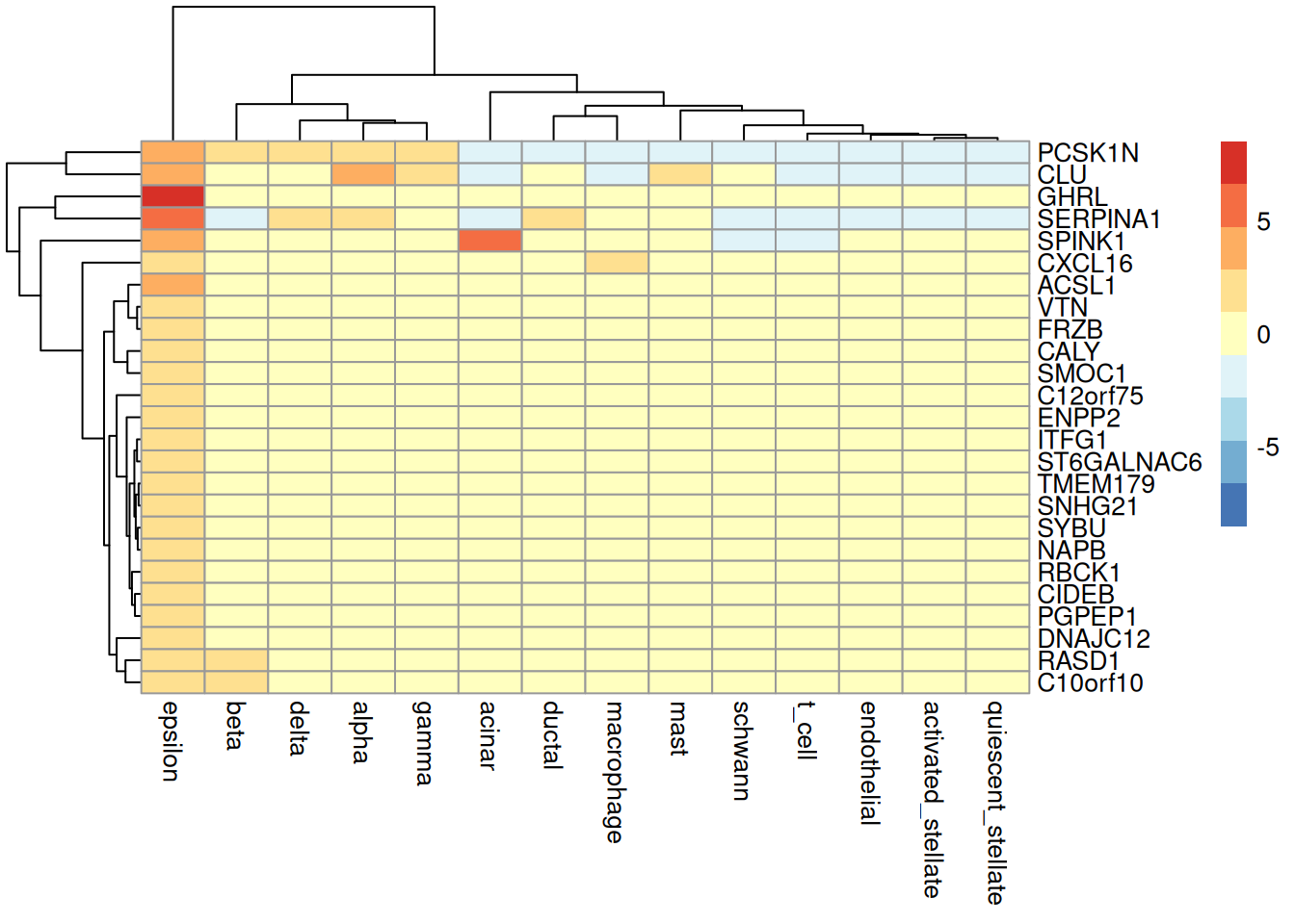
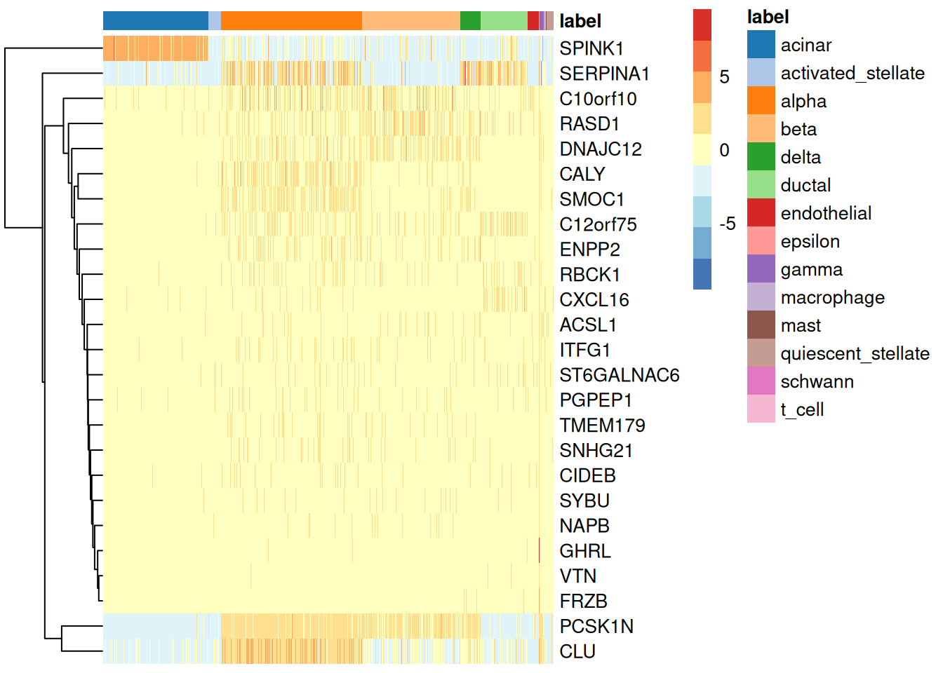
Much stronger, GHRL appears at rank 2:
- GHRL: correctly surfaces near the top
- VTN: same caveat as before, non-specific
- SERPINA1, SPINK1: pancreatic-associated but typically linked to exocrine/acinar cells rather than epsilon specifically
- PCSK1N: proprotein convertase inhibitor, plausible, since epsilon cells process peptide hormones like ghrelin, this fits the hormone-processing machinery theme even if not epsilon-exclusive
- CIDEB, ACSL1, NAPB, SYBU, CALY, RASD1: lipid handling/secretory-vesicle genes, biologically plausible for a hormone-secreting cell type but not classic textbook markers
- FRZB, ENPP2, CXCL16, SMOC1, C12orf75, TMEM179, PGPEP1, ST6GALNAC6, ITFG1, CLU, RBCK1, C10orf10: mostly uncharacterized or broadly-expressed genes for this context
min
1ordered <- chosen[order(chosen$min.logFC.cohen,decreasing=TRUE),]
2head(ordered)
 1## DataFrame with 6 rows and 19 columns
 2##            self.average other.average self.detected other.detected
 3##               <numeric>     <numeric>     <numeric>      <numeric>
 4## GHRL            9.19138    0.00164257             1     0.00131614
 5## VTN             2.74298    0.00533242             1     0.00497212
 6## FRZB            3.00081    0.01920769             1     0.01258725
 7## SYBU            2.04196    0.03471349             1     0.02799088
 8## NAPB            1.83091    0.03786699             1     0.03227985
 9## ST6GALNAC6      2.04196    0.14528431             1     0.11050636
10##            mean.logFC.cohen min.logFC.cohen median.logFC.cohen max.logFC.cohen
11##                   <numeric>       <numeric>          <numeric>       <numeric>
12## GHRL               24.18584        23.74169           24.29966        24.29966
13## VTN                28.37347        16.94799           31.87112        31.87112
14## FRZB                8.26435         6.44749            8.72608         8.72608
15## SYBU               38.59628         5.60475           18.56236        88.93492
16## NAPB                7.80530         5.37676            8.24785         9.73400
17## ST6GALNAC6         19.49805         4.07685            5.69624        88.93492
18##            rank.logFC.cohen  mean.AUC   min.AUC median.AUC   max.AUC  rank.AUC
19##                   <integer> <numeric> <numeric>  <numeric> <numeric> <integer>
20## GHRL                      1  1.000000  1.000000          1         1         1
21## VTN                       1  1.000000  1.000000          1         1         1
22## FRZB                      4  1.000000  1.000000          1         1         1
23## SYBU                      1  0.998219  0.987929          1         1         1
24## NAPB                      6  0.998446  0.990683          1         1         1
25## ST6GALNAC6                2  0.990433  0.928571          1         1         1
26##            mean.logFC.detected min.logFC.detected median.logFC.detected
27##                      <numeric>          <numeric>             <numeric>
28## GHRL                   1.53619           1.000000               1.58496
29## VTN                    1.52593           1.000000               1.58496
30## FRZB                   1.50560           1.000000               1.58496
31## SYBU                   1.46471           1.000000               1.50696
32## NAPB                   1.45248           1.000000               1.52463
33## ST6GALNAC6             1.26321           0.980891               1.22362
34##            max.logFC.detected rank.logFC.detected
35##                     <numeric>           <integer>
36## GHRL                  1.58496                   1
37## VTN                   1.58496                   1
38## FRZB                  1.58496                   1
39## SYBU                  1.58496                   1
40## NAPB                  1.58496                   1
41## ST6GALNAC6            1.58496                   1
1top.cohen.min <- rownames(ordered)[1:length(top.markers)]
2plotHeatmap( sce.baron,
3             features=top.cohen.min,
4             order_columns_by="label",
5             center=TRUE
6           )
1plotGroupedHeatmap( sce.baron,
2                    features=top.cohen.min,
3                    group="label",
4                    center=TRUE
5                  )
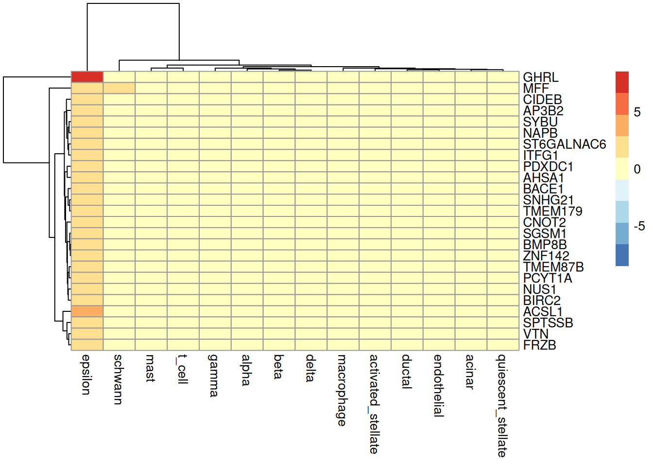
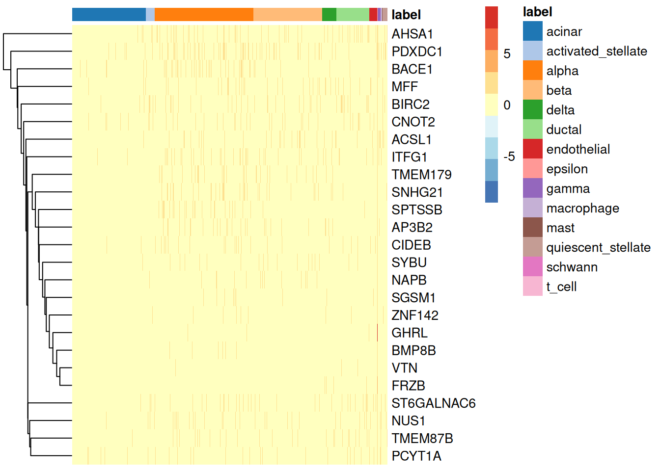
GHRL ranks #1, the strongest recovery of the canonical marker across all four lists:
- GHRL: correctly identified as the single strongest distinguishing gene
- VTN, FRZB, SYBU, NAPB, CIDEB, ACSL1: recurring, same caveats as above
- ST6GALNAC6, ITFG1, TMEM87B, SNHG21, TMEM179,
PDXDC1, PCYT1A, AHSA1, NUS1: same generic genes seen
in the
findMarkers.alllist - MFF, SPTSSB, BMP8B, SGSM1, BACE1, ZNF142, CNOT2, BIRC2, AP3B2: no established epsilon-cell association found; likely noise
compare results
 1dataset <- "Epsilon"
 2namedGenesList <- list( findMarkers.all = top.markers, findMarkers.some = top.markers.some,
 3  cohen.median = top.cohen.markers, cohen.min = top.cohen.min
 4)
 5venn.diagram( namedGenesList,
 6                  paste0(dataset, "Venn.diagram.tiff"),
 7                  fill=wes_palette("FantasticFox1")[1:length(namedGenesList)],
 8                  alpha=rep( 0.25, length(namedGenesList) ),
 9                  cex = 2.5, cat.fontface=4,
10                  category.names = names(namedGenesList),
11                  col=wes_palette("FantasticFox1")[1:length(namedGenesList)]
12                )
1## [1] 1
1log.files <- list.files('.', pattern = "*Venn.diagram.*.log", full.names = T)
2file.remove(log.files)
1## [1] TRUE
1cmd <- paste0( 'convert ', dataset, 'Venn.diagram.tiff ', dataset, 'Venn.diagram.png && rm ', dataset, 'Venn.diagram.tiff ' )
2system( cmd )
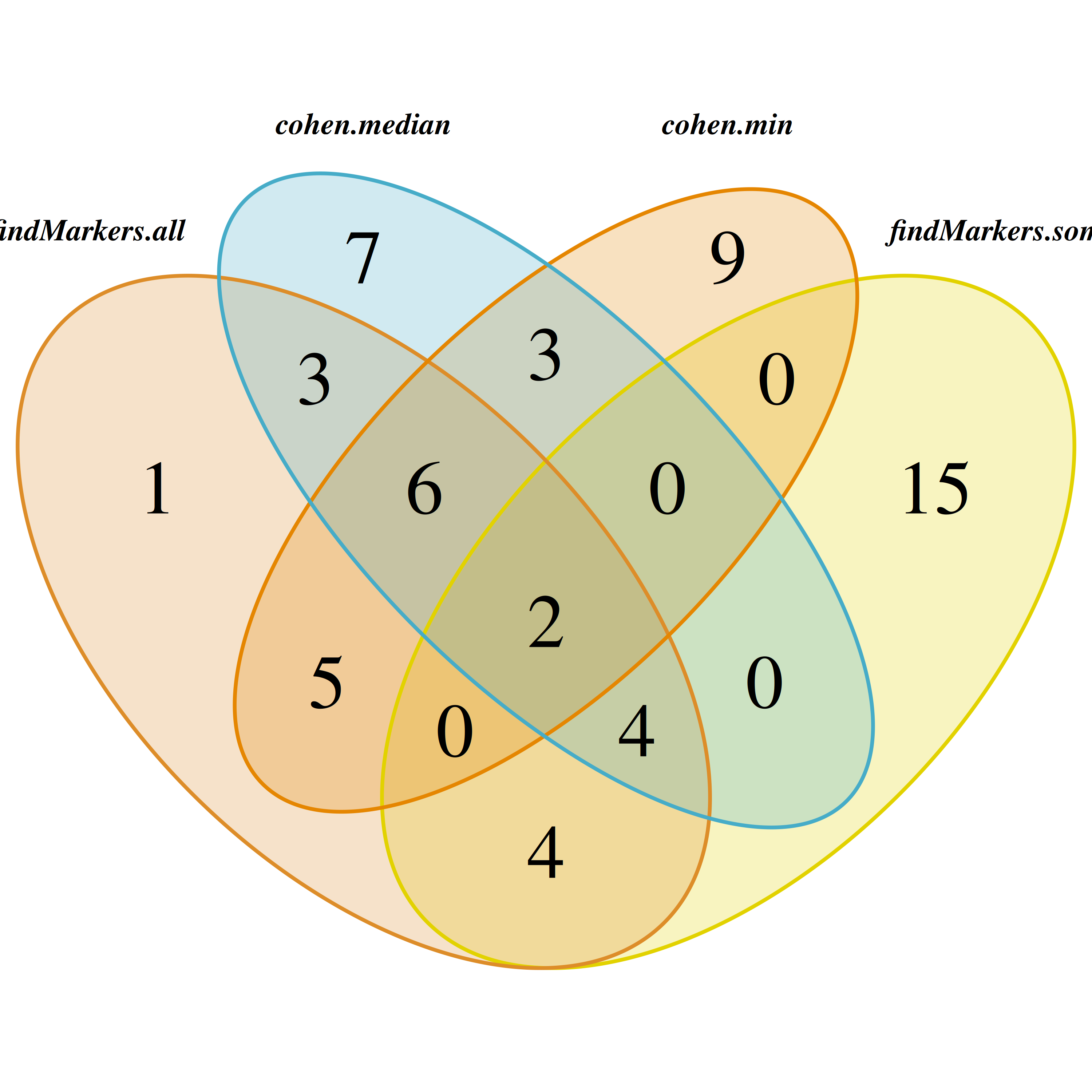
| List | GHRL rank | Overall signal quality |
|---|---|---|
findMarkers.all |
14/25 | Weak, canonical marker present but buried |
findMarkers.some |
absent | Weakest, canonical marker missing entirely |
cohen.median |
2/25 | Moderate-strong |
cohen.min |
1/25 | Strongest, canonical marker correctly top-ranked |
Key finding: on a very rare, small cluster, scoreMarkers's
effect-size-based ranking (Cohen's d) recovers the one biologically
definitive marker (GHRL) far more reliably than findMarkers's
p-value-based approach does, and counterintuitively, the "Most conservative"
(cohen.min) criterion does better than the "typical-case"
(cohen.median) one here, because GHRL's expression is so dramatically
and consistently exclusive to epsilon cells that it wins even the
strictest pairwise effect-size comparison.
The likely explanation: p-values are highly sensitive to sample
size, and with epsilon cells being such a tiny population, individual
pairwise t-tests/Wilcoxon tests lack statistical power even when the
underlying effect (expression difference) is huge, this is exactly why
GHRL can fail to reach "significant in every comparison"
(findMarkers.all) or "significant in most comparisons"
(findMarkers.some) despite being the textbook marker. Effect sizes
(Cohen's d), by contrast, don't require large sample sizes to be large
— a huge mean difference is a huge effect size regardless of n, which
is why scoreMarkers recovers it reliably even here.
Practical takeaway: this is a clean, well-documented example of
exactly the kind of divergence Baron's rare cell types were meant to
surface, findMarkers struggling with statistical power on tiny
clusters, scoreMarkers remaining robust because it isn't gated by a
significance threshold.
Conclusions
- For clearly separated clusters with enough cells both approaches work similarly, although Cohen's d seems to work slightly better.
- Cohen's d has the extra advantange of being faster (or more efficient), compare them on a dataset of hundred thousand cells and you will see.
- Things get more complicated with small of not clear clusters, see the last example.
- The number of 'good' marker genes depends on the experimental model and the specific clustering performed.
- Domain knowledge and previous information on the dataset under study is key to properly understand the clusters identity
Further reading
- "Single-cell best practices" book: From cluster differentially expressed genes to cluster annotation
- “Orchestrating Single-Cell Analysis with Bioconductor” book: Chapter 6 marker gene detection
- Seurat - Guided Clustering Tutorial: Finding differentially expressed features (cluster biomarkers)
- Lucy L. Gao double dipping example(for some reason this link is only working sometimes now)
- Wikipedia Circular_analysis